Entropy-Based Integration of Geological and Geoelectrical Parameters for Groundwater Vulnerability Assessment in Oke-Aro, Akure, Nigeria

Received 24 Nov, 2025

Accepted 25 Jan, 2026

Published 26 Jan, 2026

Background and Objective: Groundwater resources in basement complex terrains are susceptible to contamination due to the heterogeneous nature of subsurface layers. Oke-Aro community in Akure, Southwestern Nigeria, faces increasing groundwater usage without adequate vulnerability assessment. This study aimed to evaluate the aquifer vulnerability in the area to determine groundwater potability by integrating geologic and geo-electrical parameters using an entropy-based data-driven model. Materials and Methods: A total of 30 Vertical Electrical Soundings (VES) were conducted using the Schlumberger array with AB/2 spacing between 65 and 100 m. Additionally, 30 static water level (SWL) measurements were taken from hand-dug wells to validate the model. The VES data revealed 3-4 geoelectric layers correlating to topsoil, weathered layer, partially fractured basement, and fresh basement. Seven conditioning factors-lithology (L), slope (S), longitudinal resistivity (LR), overburden thickness (OLT), transverse resistance (TR), transverse resistivity (ρt), and coefficient of anisotropy (COA)-were derived and weighted using the entropy method to produce a groundwater vulnerability map (GVM). Model validation was conducted by overlaying SWL data onto the GVM. Results: The GVM classified the study area into four vulnerability zones: Very low, low, medium, high, and very high. The validation using SWL data yielded a model accuracy of 56.25%. Areas with high vulnerability corresponded with shallow water levels, indicating potential susceptibility to surface contamination. Conclusion: The study demonstrates the applicability of entropy-based models in groundwater vulnerability assessment within complex geologic settings. Despite moderate validation accuracy, the approach offers a valuable framework for preliminary vulnerability mapping. Future studies should incorporate additional hydrochemical and land use data for improved accuracy.

INTRODUCTION

Water, an indispensable resource, is needed for the survival and development of all species; man, animal and plant. Human activities such as agricultural practices, industries, and domestic consumption depend solely on availability¹ of water resources. Despite its importance, over-extraction, or excessive pumping of groundwater, can lead to depletion of aquifers, causing water shortages and land subsidence. Also, groundwater contamination through agricultural runoff, industrial waste, and septic systems could lead to water-borne diseases such as Cholera. Climate change is also altering precipitation patterns and increasing the frequency and intensity of droughts, which can affect groundwater availability and quality. The increasing rate of groundwater contamination, especially in developing countries, has become a problem that has recently gained the attention of professionals, academic scholars, and stakeholders in the management of groundwater resources in recent times. Water pollution concerns have become alarming as a result of rapid and broad population growth, irregular planning, urban sprawl, various land use classification patterns nd systems, and inadequate sewage disposal systems^2-4. The generation of waste is an indispensable characteristic of life. Pollutants are aqueous liquids called leachate, which is formed when rain falls on waste, percolates into the waste, and picks up contaminants as it seeps downwards. Water conservation, pollution control, and aquifer vulnerability zonation is essential for sustainable groundwater management.

The electrical resistivity (ER) method is one of the most widely used methods in solving groundwater contamination problems⁴. Subsurface contamination can be detected, and the overall vulnerability of the study area can be determined using resistivity methods⁵. Previous studies have investigated groundwater vulnerability in similar geological settings using Multi-Criteria Decision Analysis (MCDA) as a viable tool^6-13.

The groundwater vulnerability of the Northwest Region of Akure, Southwest Nigeria, has been evaluated¹⁴ using lithology, elevation, and four geoelectrically derived factors. The aquifer vulnerability model map was created by integrating the six parameters: Lithology, elevation, topsoil (resistivity and thickness), and weathered layer (resistivity and thickness) using an additive model. The aquifer vulnerability model map indicated that 30% of the area is of low vulnerability, 65% is of moderate vulnerability, and 5% is of very low vulnerability. Using the DRASTIC MODEL, Mogaji et al.¹⁵ conducted a study on groundwater vulnerability in the Southern Region of Perak, Malaysia¹⁵. Analytical Hierarchy Process (AHP) was used to incorporate seven DRASTIC parameters. A groundwater vulnerability map of the area was created using the integrated parameters. Five zones were identified in the study area: Non vulnerability (NV), very low vulnerability (VLV), low vulnerability (LV), moderate vulnerability (MV) and high vulnerability (HV).

Groundwater vulnerability to pollution was evaluated using the Fuzzy Analytic Hierarchy Process (FAHP) combined with the DRASTIC method in Suhut Plain, Southwest Turkey⁷. The study revealed that the most effective impact parameters found were the impact of the vadose zone and net recharge whereas the soil media had no significant impact in the vulnerability map, DRASTIC factors were rated using FAHP and finally, the information was integrated using single-parameter sensitivity analysis (SPSA) and areas with very high and high vulnerable zones due to high pollution potential of intensive agricultural activities were identified. Groundwater quality and portability of Aule Area in Akure Metropolis, South Western, Nigeria have been evaluated¹⁴. Twenty-one water samples were collected from wells for chemical analysis. Based on the analytical results, it was observed that the groundwater within the study area is of good quality and hence suitable for drinking and other domestic purposes. However, appropriate remedial treatment is recommended for the groundwater at the locations where trace elements are at the upper limit of WHO recommended. Water analysis was employed to examine the effect of automobile repair workshops on the water quality of a selected area in Ado Ekiti, Nigeria¹⁵. The results portrayed evidence of water contamination. It was concluded that both the surface and well water around the study areas are not fit for consumption due to the high concentration of some elements and compounds.

Assessment of aquifer vulnerability using multi-criteria decision analysis was done in parts of Akure Southwestern Nigeria¹⁶. The study considered four factors: Topsoil Resistivity (TSR), Longitudinal Conductance (LC), Hydraulic Conductivity (HC), and Thickness of the Layer overlying the Aquifer (TLOA).

Normalized weights were assigned to parameters with the help of AHP and a groundwater vulnerability map of the area was generated. This map was categorized into five zones: Very low, low, moderate, high, and very high. A larger percentage of the area had moderate vulnerability to contamination. Similarly, different databases, namely geophysical, hydrological, weather, soil, and remote sensing-derived parameters were integrated to evaluate the vulnerability of groundwater to contamination from surface pollution using the Analytic Hierarchy Process (AHP) technique¹¹. The study revealed better efficiency of the developed DRASTICALLY model against the conventional DRASTIC model when validated using water chemical analysis data.

The ENTROPY technique adopted in this study to integrate lithological, elevation, and geo-electrically derived parameters involves assigning criterion weight based on their variability and importance and rating them using the Simple Additive Weighting (SAW) to produce the groundwater Vulnerability Index (GVI) model map of the study area. The static water level of hand-dug wells in the study area was used for the validation of the groundwater vulnerability model map. The specific objectives of this study are to identify the subsurface geo-electric sequence underlying the study area, determine the groundwater vulnerability conditioning parameters; slope, aquifer Overlying layer thickness, lithology, traverse resistance, longitudinal resistivity, coefficient of anisotropy, and traverse resistivity, produce the groundwater vulnerability model map (GVM) of the area using the Entropy Model, identify different vulnerability zones in the study area, which will aid effective groundwater resources management, and validate the groundwater vulnerability model map (GWVM) using the static water level (SWL) of the wells in the study area.

MATERIALS AND METHODS

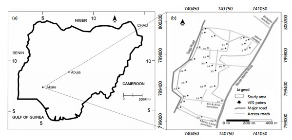
Location of the study area: The Study area is located within Akure Metropolis, Southwestern Nigeria. Located within a town popularly known as Oke-Aro Akure, the area is situated within geographic grids of 740432-740958 m (Eastings) and 799005-800101 m (Northings) defined by the WGS-84 31N datum of the Universal Traverse Mercatum (UTM). The study area is accessible through the Akure-Idanre road and many other interconnected minor roads and footpaths (Fig. 1).

The study area is moderately undulating with surface elevations that range between 330 and 370 m above mean sea level. The southern part of the study is at a lower elevation, while the northern part is at a higher elevation. The study area has two major seasons of the year: Wet (April to October) and dry (November to March). The mean rainfall ranges between 1500 and 2100 m. For the annual temperature, it ranges from 21 to 29°C¹⁷, sometimes extending to 32°C. Humidity is relatively high. The coldest month of the year is around August, with an average low temperature between the range of 21°C, and the hottest month of the year is around March, with an average temperature within 32°C. The study area was investigated during the rainy season of the year (May, 2024).

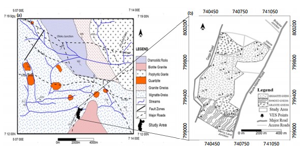
The area around the Akure Metropolis is underlain by six petrological units: Migmatite-gneiss, granite-gneiss, quartzite, charnockite, biotite gneiss, and porphyritic granite¹⁸ of the Precambrian basement complex of Southwestern Nigeria (Fig. 2a), Three lithological units were identified in the area: the migmatite-gneiss, banded-gneiss, and granite-gneiss, with the migmatite-gneiss being the most widespread, covering more than half of the research area (Fig. 2b). The was survey was done to obtain information such as the geology of the study area, drainage pattern, accessibility, vegetation, topography, and possible outcrops in the research area. This acquired information was used to generate the base map of the research area that helped in crafting an excellent geophysical survey plan.

Data acquisition, processing, and interpretation: The electrical resistivity method was employed in this research, while the Vertical Electrical Sounding (VES) field technique (Schlumberger electrode configuration) was used for the data acquisition. A total of thirty VES positions were occupied across the research area (Fig. 1b) with half-current electrode separation (AB/2) ranging from 1-100 m. The VES data were acquired along roadsides, available undeveloped plots of land, and linear routes between houses. The data acquisition points were geo-referenced with the aid of the Global Positioning System (GPS). The acquired resistivity data were presented as field curves which is a plot of apparent resistivity (pa) values against half-current electrode spacing¹⁹.

Fig. 1(a-b) Location maps: (a) Ondo State map showing Akure (b) Map of the study area

Fig. 2(a-b): (a) Geological map of Akure18 and (b) Geological map of the study area

The filed curves were quantitatively interpreted through partial curve matching with the use of 2-layer master curves and corresponding auxiliary curves to obtain primary geoelectric parameters involving the initial estimates of resistivity and thickness values of various geoelectric layers at each VES point^20-22. These geoelectric parameters from manual interpretation were used as initial starting models in the computer-assisted iteration using WinResistTM Software, which was developed²³ to generate iterated curves from which the primary geoelectric parameters were determined. The first and second-order geoelectrically derived parameters obtained from the VES consist of the following; longitudinal resistivity (LR), overlying layer thickness (OLT), traverse resistance (TR), traverse resistivity (ρt) and coefficient of anisotropy (CoA).

Groundwater vulnerability conditioning factors (GWVCFs) thematic layers
Lithology (L): The study area consists of three distinct geological units; Migmatite-Gneiss, Banded-Gneiss, and Granite-Gneiss. In a typical basement complex terrain characterized by crystalline rock, the underlying rock tends to be brittle and prone to fracturing and this results in high transmissivity and percolation of contaminants, as well as higher levels of porosity and permeability in the weathered/fractured basement of the rock²⁴.

Slope (S): Elevation influences surface run-off. Elevation reduces the possibility that a contaminant may flow off or remain on the surface in one location long enough to permeate the underlying aquifer unit²⁵. Water is more likely to penetrate low-slope locations. Surface runoff is reduced in these regions, allowing a significant chance of pollutant infiltration, while areas with steep slopes promote massive amounts of runoff with short residence time for infiltration²⁶. High infiltration makes groundwater more vulnerable, while low infiltration makes groundwater less vulnerable.

Longitudinal resistivity (LR): Longitudinal resistivity refers to the resistance of the subsurface materials to the flow of groundwater along the horizontal direction. Higher LR values suggest low porosity, low permeability and low water content along the horizontal direction^20-27. High longitudinal resistivity can limit the infiltration of contaminants from surface water into the subsurface, thereby reducing the vulnerability of groundwater to contamination²⁸.

Overlying layer thickness (OLT): The overlying layer thickness (OLT) refers to the vertical distance the contaminant or pollutant will cover before getting to the groundwater. The thicker the OLT the lower the vulnerability of the aquifer layer¹¹.

Traverse resistance (TR): Traverse resistance (TR) is an important geoelectric parameter in assessing aquifer vulnerability in basement environments. Higher TR values indicate better protection, whereas lower values indicate greater vulnerability to pollution.

Traverse resistivity (ρt): A high traverse resistivity value depicts low vulnerability to contamination because high-resistive materials inhibit the flow of water and contaminants. These areas tend to be less vulnerable to surface contamination since water and pollutants struggle to penetrate and reach the aquifer. For low traverse resistivity value, indicates that the subsurface materials allow easier infiltration of water, which also makes it easier for contaminants to percolate down to the groundwater. Such areas are more prone to contamination from surface activities, including agricultural runoff, industrial pollutants, and sewage.

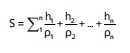
Coefficient of anisotropy (CoA): The coefficient of anisotropy refers to the degree of inhomogeneity of the subsurface lithology, and hence an indirect measure of the degree of fracturing (24). The coefficient of anisotropy is a second-order geoelectric parameter calculated from two geoelectric fundamental parameters: Layer resistivity (ρ) and thickness (h). Other second-order geoelectric parameters involving total unit longitudinal conductance (S); total traverse unit resistance (T); average longitudinal resistivity (; and the average transverse resistivity were used in the computation of the coefficient of anisotropy as shown in equations 1-5 where n is the number of geoelectric layers and h is the thickness of each geoelectric layer^29-31. A low coefficient of anisotropy value implies a low degree of fracturing and thus suggests low groundwater vulnerability, while a relatively high coefficient of anisotropy indicates a significant level of fracturing and thus suggests a high potential for groundwater contamination³².

For n layers, the total longitudinal conductance (S) is formatted as Eq. 1 (20):

(1)

Where:

h₁ is the thickness of 1st layer 1, h₂ is the thickness of 2nd layer 2 and h_n is the thickness of nth layer. Similarly ρ₁ is the resistivity of 1st layer 1, ρ₂ is the resistivity of 2nd layer 2 and ρ_n is the resistivity of nth layer

Hile the total transverse resistance (T) is formatted as Eq. 2 (20):

(2)

The average longitudinal resistivity is derived from Eq. 1 and formatted as equation 3 (20):

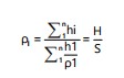(3)

And the average transverse resistivity (ρ_t) is calculated from Eq. 2 and formatted as eq. 4 (20):

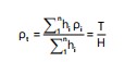(4)

Where:

H is the total thickness of all the subsurface layers

The coefficient of anisotropy, λ, is calculated from Eq. 3 and 4 and formatted as eq. 5 (20):

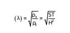(5)

For an isotropic layer, ρ_t = ρ_l and λ = I

Entropy technique: The entropy technique is a data-driven approach that was first proposed by Shannon³³ and modified by Xu et al.³⁴ and Shevyrev and Carranza³⁵. The entropy method is an object-driven (non-expert) approach that involves determining the weight values of individual indicators by calculating the entropy and entropy weight³⁶. The method is based on the idea of discreet probability distribution where uncertainty is depicted with broad distribution³⁷ and since entropy is the measure of a system’s disorder, it can be used to extract useful information from a given data³⁸.

The difference in the values of the evaluating objects on a criterion has a direct effect on the entropy. Entropy has been used widely in literature by several researchers in various fields of science^39-43, the results showed appreciably good prediction accuracy. The method determines the weights of thematic layers by assuming that there is a set of m feasible alternatives, Ai (i = 1, 2, ..., m) and n evaluation criteria Cj (j = 1, 2, ..., n) in the problem⁴². The formulation of the ENTROPY technique can be described in a series of steps as follows^42,43.

Step 1: A decision matrix (X_ij) is initially created as formatted in Eq. 6, the essence is that it shows the performance of different alternatives relative to various criteria.

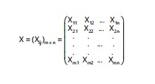(6)

for i = 1, 2, …, m; j = 1, 2, …, n

Where:

	Xim	=	Feasible alternative
	Xjn	=	Evaluation criterion
	m	=	Number of alternatives
	n	=	Number of criteria

Step 2: Normalization of the decision matrix (r_ij) as formatted in Eq. 7. This is done by dividing each criterion value (x_ij) by the total arithmetic column sum of the criteria

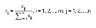(7)

Step 3: Calculation of entropy values (e_j) as formatted in Eq. 8, 9:

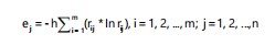(8)

Where:

(9)

Step 4: Calculation of entropy weight (w_j) as formatted in Eq. 10:

(10)

Where:

The dj values, entropy (e_j), and entropy weight (w_j) for each parameter are represented in Table 1. The result shows that the slope of the study area has the lowest Entropy weightage of 0.13321414 and traverse resistance has the highest weightage of 0.162194288.

Rating of GWVCFs thematic layers: Each of the conditioning factors influencing the study area's groundwater vulnerability was assigned a rating (R) of 0.2-1.0 (Table 2). The rating was used to estimate the study area’s groundwater vulnerability index (GVI).

Table 1:

The dj values, entropy values, and entropy weight values of conditioning factors

Parameter	Dj values	Entropy	Entropy weight
Slope	0.2962564	0.7037436	0.1332141
Total overlying thickness	0.3392433	0.6607567	0.1525436
Lithology	0.298962	0.701038	0.1344307
Traverse resistance	0.3607057	0.6392943	0.1621943
Longitudinal resistivity	0.3164259	0.6835741	0.1422835
Coefficient of anisotropy	0.2964141	0.7035859	0.133285
Traverse resistivity	0.3159037	0.6840963	0.1420487

Table 2:

Normalized weight and rating for classes of factors

Parameter	Classes	Vulnerability potential for groundwater	Rating (unstandardized values)	Normalized weight (W)
Slope	330-338	Very high	1	0.1332141
	339-346	High	0.8
	346-354	Medium	0.6
	354-360	Low	0.4
	>360	Very low	0.2
Total overlying thickness	<1.5	Very high	1	0.1525436
	1.5-3.0	High	0.8
	3.0-4.5	Medium	0.6
	4.5-6	Low	0.4
	>6	Very low	0.2
Lithology	Granite Gneiss	0.23	0.4	0.1344307
	Banded Gneiss	0.37	0.2
	Migmatite-Gneiss	0.4	0.2
Traverse resistance	0-59	Very low	0.2	0.1621943
	60-119	Low	0.4
	120-249	Medium	0.6
	250-449	High	0.8
Longitudinal resistivity	0-59	Very low	0.2	0.1422835
	60-119	Low	0.4
	120-249	Medium	0.6
	250-449	High	0.8
	>450	Very high	1
Coefficient of anisotropy	<1.0	Very low	0.2	0.133285
	1.0-1.07	Low	0.4
	1.08-1.16	Medium	0.6
	1.16-1.23	High	0.8
	≥1.24	Very high	1
Traverse resistivity	0-59	Very low	0.2	0.1420487
	60-119	Low	0.4
	120-249	Medium	0.6
	250-449	High	0.8
	>450	Very high	1

Groundwater vulnerability index (GVI) estimation: The groundwater vulnerability index (GVI) is the product of the assigned weight "W" and the ratings 'R' of all the factors used in the evaluation. The technique used to estimate GVI is referred to as the "weighted linear average technique". This technique is typically described in terms of weightings (W) for each factor, as well as rating scores (R) for all options in relation to each.

Equation 11 below describes the groundwater vulnerability index (GVI):

(11)

Where:

	Wi	=	Weight (w) of parameter "i"
	R	=	Parameter;s rating score

Equation 12 represents the vulnerability index equation for each location, which was estimated using the weights (W) and ratings (R) of each factor:

(12)

where, subscript S, Li, OLT, TR, ρl, COA, and ρt are the slope from elevation, lithology, overlying layer thickness, traverse resistivity, longitudinal resistivity, coefficient of anisotropy, and traverse resistivity weight and rating, respectively.

RESULTS

The VES data identified three to four geo-electric layers across the area, corresponding to four subsurface layers: Topsoil, weathered layer, partially weathered basement, and presumed fresh basement. The first and second order parameters derived from the VES results are shown in Table 3.

Three curve types were delineated across the study area; A, H, and KH. The frequency of the typical curve types obtained from the area shows that curve types H and KH are the predominant curve types in the area. The curve types in the study area can be divided into two groups based on the confinement of the target aquifer(s). Group 1 curve types include KH, with the aquifer layer(s) overlaid by a confining layer. The layer above it well protects the aquifer layer in this category. Group 2 contains the curve types A and H. This group’s aquifer layer(s) are unconfined, making them vulnerable.

Table 3:

Summary of first and second order parameters

VES points	Easting	Northing	S	L	(OLT)	(TR)	LR	CoA	ρt
1	740958	799875	363	MG	1	46.2	46.2	1	46.2
2	740917	799851	358	MG	7.1	1108.6	94	1.29	156
3	740915	799923	356	MG	1.6	132.8	83	1	83
4	740949	799972	351	MG	1.1	201.3	183	1	183
5	740905	799996	360	MG	0.9	88.2	98	1	98
6	740568	800101	365	GG	0.9	127.8	142	1	142
7	740563	800056	345	GG	0.7	140	200	1	200
8	740648	800018	341	GG	1.1	57.2	52	1	52
9	740517	799883	348	GG	0.9	20.7	23	1	23
10	740589	799872	347	MG	1	120	120	1	120
11	740756	799920	366	MG	1.1	44	40	1	40
12	740745	799868	352	MG	1.6	105.6	66	1	66
13	740589	799772	355	MG	0.9	128.7	143	1	143
14	740626	799663	347	MG	2.1	510.3	243	1	243
15	740657	799597	350	MG	0.8	147.2	184	1	184
16	740730	799659	353	MG	0.7	81.9	117	1	117
17	740648	799411	335	MG	0.9	114.3	127	1	127
18	740564	799413	337	MG	1.2	45.6	38	1	38
19	740529	799274	335	GG	0.8	94.4	118	1	118
20	740411	799298	331	BG	0.9	141.3	157	1	157
21	740713	799235	342	GG	1	95	95	1	95
22	740655	799005	343	BG	1.2	76.8	64	1	64
23	740535	799046	337	BG	1.1	101.2	92	1	92
24	740348	799160	338	BG	6.7	683.4	102	1	102
25	740380	799229	335	BG	1.5	70.5	47	1	47
26	740400	799460	347	MG	1.2	337.2	281	1	281
27	740332	799385	351	MG	1	168	168	1	168
28	740389	799599	345	MG	1	204	204	1	204
29	740471	799741	345	MG	2.5	303.5	96	1.13	121
30	740576	799696	344	MG	1	136	136	1	136
VES: Vertical electrical sounding, Easting and Northing are coordinates (m), S: Slope (°), L: Lithology (derived from geoelectric interpretation), OLT: Overburden thickness (m), TR: Transverse resistance (Ω·m2), LR: Longitudinal resistivity (Ω·m), CoA: Coefficient of anisotropy (dimensionless), ρt: Transverse resistivity (Ω·m) and First-order parameters are directly obtained from VES interpretation, whereas second-order parameters are computed from first-order resistivity and thickness values

Fig. 3: Elevation map of the study area

Fig. 4: Overburden layer thickness map of the study area

Aquifer vulnerability assessment: The assessment of groundwater vulnerability in the study area was conducted utilizing data from multiple sources. Slope data from surface elevation, lithological data from the geological map, and five geoelectrically derived parameters (overlying layer thickness (OLT), longitudinal resistivity (LR), traverse resistance (TR), coefficient of anisotropy (CoA), and traverse resistivity (ρt)) were combined for the aquifer vulnerability assessment (Table 4).

Table 4:

Readings of the static water measurement

Wells No.	Easting	Northing	Static water level depth (m)
1	740957	799867	6
2	740940	799841	6.1
3	740889	799843	6.4
4	740888	799843	6.6
5	740865	799888	7
6	740879	799906	6.9
7	740607	800097	3.5
8	740586	800027	5.05
9	740657	800011	3.2
10	740792	799899	4.18
11	740598	799883	3.4
12	740600	799802	2.95
13	740590	799684	1.85
14	740652	799603	3.43
15	740674	799582	1.95
16	740638	799663	3.2
17	740734	799636	2.4
18	740494	799725	5.16
10	740445	799704	5.15
20	740423	799655	4.7
21	740416	799643	4.45
22	740352	799419	2.67
23	740392	799466	3.4
24	740349	799355	1.65
25	740360	799153	2.7
26	740362	799171	2.48
27	740515	799050	3.32
28	740529	799046	3.57
29	740634	799258	1.3
30	740533	799280	2.7

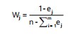
Slope (elevation) map: The elevation map (Fig. 3) shows that the study area is moderately undulating, with surface elevations ranging from 331 to 366 m. During precipitation, surface water flows from northwest to southwest. Infiltration decreases as elevation rises, and increases as elevation falls. High infiltration makes groundwater more vulnerable, whereas low infiltration makes groundwater less vulnerable. The elevation map (Fig. 3) classified the area into five zones (very high, high, medium, low, and very low) based on the developed class interval shown on the thematic map.

The produced thematic map shows that the Southern Region of the study area is more vulnerable, showing a variation of very low to low elevation. The southeastern region is extremely vulnerable to groundwater, as is the lower part of the south-central region, which has a low elevation of 338-46 m. Moderate elevation falls within the class of 346-354 m in the Northern part of the central region, indicating medium groundwater vulnerability and extending to the study area’s northwest. However, there is an isolated region in the northwest direction with a low elevation (338-346 m). The northwestern region of the study area has a range of elevations (354-360 m), indicating low vulnerability, and the highest elevation (over 360 m), indicating the lowest vulnerability region in the study area.

Lithology map: The study area contained three rock types: Migmatite gneiss, banded gneiss, and granite gneiss. The geological map of the study area (Fig. 2b) shows that Migmatite Gneiss occupies a larger area than the other rock types present in the study area. Migmatite gneiss weathers into a variety of materials, often resulting in clayey to sandy soils. The degree of weathering of subsurface rocks can affect groundwater vulnerability. Charnockite areas, unlike Migmatite gneiss area may be associated with low to moderate vulnerability because they yields essentially clayey weathering products, particularly from more granitic components, have high porosity but low permeability, limiting groundwater flow. The metamorphic bands may cause fractures that allow water to move, but the weathered material’s clay content tends to limit infiltration.

Fig. 5: Traverse resistance map of the study area

Banded gneiss weathers into clay and silt, contributing to its low vulnerability. The foliated structure can cause fractures or joints, which allow for some water movement. However, like charnockitic rocks, the weathered material is primarily composed of clayey components with low permeability, which reduces groundwater infiltration and flow. The permeability is most likely low to moderate due to the nature of weathered products and the foliated structure, which may trap water rather than allow free flow.

Granite gneiss, like granite, weathers to form sandy soils with higher porosity and permeability than clay-rich rocks. This means that areas with granite gneiss may be moderately to highly vulnerable due to the increased permeability of the weathered sand, which allows for easier water infiltration into the subsurface. Granite gneiss’s moderate to high permeability allows for faster infiltration of water, making it more vulnerable to contamination if pollutants are present.

Overlying layer thickness (OLT) map: The area’s overlying layer thickness map (Fig. 4) depicts the isopach of the layer(s) that lie above the aquifer layer. The thickness of the overlying layer varies between 0.7 and 7.1 m. The OLT map (Fig. 4) shows that the aquifer overlying material in the study area is generally thin (less than 3 m) in the enclosed part of the Northwestern region, as well as the Southeastern, Western, and Eastern parts of the study area, implying that the aquifer in these areas is extremely vulnerable. The OLT in the Southwestern, Northeastern and in some isolated Western parts of the study area ranges in thickness from 3 to 7.1 m. The thicker the overlying layer the lower the vulnerability. Because the overlying layer is generally thin, potential contaminants will infiltrate easily from the surface to the aquifer unit below, and the underlying aquifer units may become contaminated.

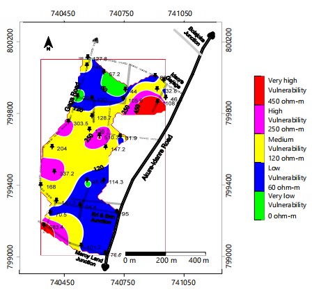
Traverse resistance (TR) map: The traverse resistance map of the study area (Fig. 5). Traverse resistance value ranges from (20.7-1108.6) Ωm. The traverse resistance map shows the spatial variation of the traverse resistance of the study area, which falls into the category of five zones. These zones are also classified to their degree of vulnerability and are stated as follows; very low vulnerability (0-59 Ωm), low vulnerability (60-119 Ωm), medium vulnerability (120-249 Ωm), high vulnerability (250-449 Ωm), very high vulnerability (greater than or equal to 450 Ωm).

Fig. 6: Longitudinal resistivity map of the study area

Fig. 7: Coefficient of anisotropy map of the study area

Traverse resistance (TR) provides valuable insights into the protective capacity of the aquifer against contaminant infiltration in basement complex environments. The Southern Region of the map depicts a range of medium to high vulnerability with the southeastern direction of the map depicting low aquifer vulnerability while the South-Western part is laid by a range of medium to very high resistivity values. The central region of the map shows medium resistivity values, with a pocket of high resistivity values which implies that this portion of the study area is moderately protected and moderately vulnerable to groundwater contamination. The North-Western part of the study area shows that this portion is less prone to vulnerability while the North-Western portion is more vulnerable due to the range of medium to high resistivity values present in the region.

Fig. 8: Transverse resistivity map of the study area

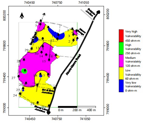
Longitudinal resistivity (LR) map: The longitudinal resistivity map (Fig. 6) shows that the spatial variation of the ρl in the study area is divided into five zones (very low, low, medium, high, and very high) with values ranging from 0-59, 60-119, 120-249, 250-449, and 450 Ωm and above. High longitudinal resistivity indicates that the subsurface materials are less permeable, which means they impede the vertical movement of water and contaminants. This acts as a protective barrier, reducing the likelihood of surface pollutants reaching groundwater. Low longitudinal resistivity indicates a higher risk of groundwater contamination because conductive materials such as saturated layers facilitate the flow of water (and dissolved contaminants) downwards toward the aquifer. The longitudinal resistivity map shows that the southern region of the study area has low resistivity values, indicating that this region is less vulnerable. The central region of the map displays a range of medium resistivity values, indicating that this portion of the study area will have a moderately high likelihood of groundwater contamination. The upper northern region of the map is dominated by low resistivity values, with a pocket of very low and medium resistivity values running through it.

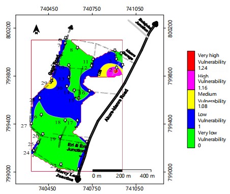
Coefficient of anisotropy (CoA) map: The anisotropy coefficient is important in determining aquifer vulnerability. Figure 7 depicts a map of the coefficient of anisotropy of the study area, which ranges from 1-3.51. The spatial distribution shows that the generated coefficient of anisotropy values from the study area is divided into five zones (very low, low, moderate, high, and very high) using the Natural Breaks Approach⁴². Different colors were used to indicate various zones ranging from green to blue, yellow to Magenta, and red, which correspond to zones of very low (0-1), low (1.1-1.08), moderate (1.081-1.16), high (1.161-1.24), and very high (1.241 and above) coefficient of anisotropy. The southern and northwestern flanks have very low anisotropy coefficient values, while the central region has low anisotropy coefficient values and the north-eastern flank has low to high anisotropy coefficients. The high coefficient of anisotropy values indicates that the fracture system must have extended in all directions with varying degrees of fracturing; this may promote good water-holding capacity from different directions of the fracture(s) within the rock, resulting in higher porosity. On the other hand, a low coefficient of anisotropy may result from unidirectional fracture, which may not produce a high groundwater yield. Areas with high coefficients of anisotropy make the area's aquifer units vulnerable to polluting fluids, and vice versa.

Fig. 9: Groundwater vulnerability map of the study area

Table 5:

Validation result of the groundwater vulnerability map and static water level map

S/N	Static water level	Static water level vulnerability (Rating)	Groundwater vulnerability (Rating)	Coincide
1	6	Very low-low	Medium	No
2	6.1	Very low-low	High	No
3	6.4	Very low-low	High	No
4	6.6	Very low-low	High	No
5	7	Very low-low	High	No
6	6.9	Very low-low	High	No
7	3.5	Medium-high	Medium	Yes
8	5.05	Low-medium	Medium	Yes
9	3.2	Medium	Medium	Yes
10	4.18	Medium	Medium	Yes
11	3.4	Medium	Medium	Yes
12	2.95	High	High	Yes
13	1.85	High	High	Yes
14	3.43	Medium-high	High	Yes
15	1.95	High	High	Yes
16	3.2	Medium-high	High	Yes
17	2.4	High	High	Yes
18	5.16	Low-medium	High	No
19	5.15	Low-medium	High	No
20	4.7	Low	High	No
21	4.45	Medium-high	High	Yes
22	2.67	High	High	Yes
23	3.4	Medium-high	High	No
24	1.65	High	High	Yes
25	2.7	High-very high	Medium	No
26	2.48	High	Medium	Yes
27	3.32	Medium-high	Medium	Yes
28	3.57	Medium-high	Medium	Yes
29	1.3	Very high	Medium	No
30	2.7	High	Medium	No

Fig. 10: Validation map of the study area using SWL

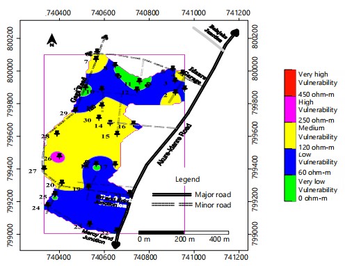
Traverse resistivity (ρ_t) map: The traverse resistivity map (Fig. 8) shows that the spatial variation of the ρt in the study area is divided into five zones (very low, low, medium, high, and very high) with values ranging from 0-59, 60-119, 120- 49, 250-449, and 450 Ωm and above.

The traverse resistivity map shows that the Southern and Northern Region of the map is characterized by low resistivity values; the Central Region of the map is characterized by a medium vulnerability with a pocket of high resistivity values at the Central West.

A high traverse resistivity value depicts low vulnerability to contamination because high-resistive materials inhibit the flow of water and contaminants. These areas tend to be less vulnerable to surface contamination since water and pollutants struggle to penetrate and reach the aquifer. For low traverse resistivity value, indicates that the subsurface materials allow easier infiltration of water, which also makes it easier for contaminants to percolate down to the groundwater. Such areas are more prone to contamination from surface activities, including agricultural runoff, industrial pollutants, and sewage.

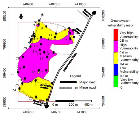
Groundwater vulnerability map (GVM): The final index from each method was classified into five different classes (Fig. 9). The Surfer 13 software was used to generate the groundwater vulnerability map from the groundwater vulnerability index (Table 3). The study was divided into five data categories: Very low, low, medium, high, and extremely high aquifer vulnerability zones.

The highly vulnerable zones (poor aquifer protective capacity) were observed in the central part of the study area and it extends to the northeastern region, ranging from high to moderate zones in this region. According to the study area’s geology, this region hosts migmatite Gneiss rock type. The Southern and Northwestern regions of the study area depict moderately vulnerable zones with banded gneiss and Granite gneiss as the major rock types in these regions.

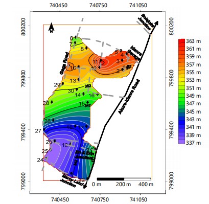
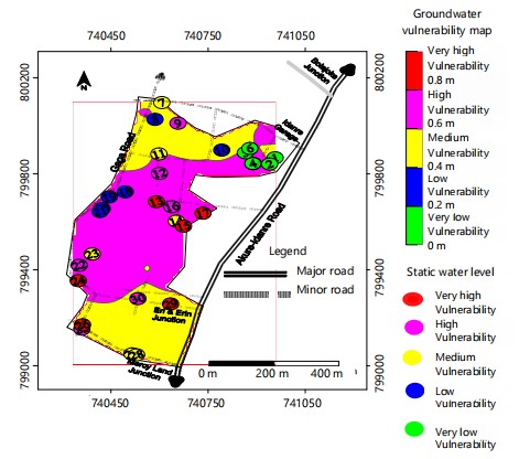
Validation map: Static water level measurement was taken from 30 wells within the study area to determine its depth to the top of the water table and the well inventory data was gathered based on these sampled wells. This consists of the coordinates and static water level for each of the wells (Table 4 and 5). The Global Positioning System (GPS) was used to acquire the coordinates at each well. The Validation map was created by plotting static water level values from well information on the developed groundwater vulnerability map (GVM) to assess the model's accuracy. Comparisons between the groundwater vulnerability zone classes and the static water level (Table 4) in the study area were done to establish the degree of correlation of the GVM and the validation map, and observing the percentage agreement using Eq. 13⁴⁰:

(13)

The static water level map (Fig. 10) showcases the distribution of the vulnerable wells based on the depth of their static water level. The five zones are distinguished by red (0-1.5 m; very high vulnerability), magenta (1.5-3 m; high vulnerability), yellow (3-4.5 m; medium vulnerability), blue (4.5-6 m; low vulnerability); green (6 m and above; very low vulnerability).

The percentage of the accuracy calculation for the entropy model can be obtained as follows:

Total number of well analyzed = 30

Number of wells where the vulnerability coincides = 17

Number of wells where the vulnerability does not coincide = 13

On this basis, the conceptual model gives an accuracy of 56.25% which is considered a fairly good prediction.

DISCUSSION

This study integrated geological and geo-electric parameters to assess groundwater vulnerability in Southwestern Akure with the aid of entropy-weighted analysis. This study revealed that aquifer vulnerability is high in the central part of the study area, an area that corresponds to about 60% of the area, while the Northern and Eastern flanks of the area which constitutes about 40% of the area are of moderate vulnerability. The zones of very low to very high vulnerability, with higher risk areas majorly in the migmatite gneiss region. This reinforced the generally accepted opinion that older rocks such as migmatite gneiss, granite gneiss and banded gneiss with highly fractured and faulted rock are more favourable for groundwater accumulation^{15,16,21,22,24}. Cosequently, older rocks with highly fractured and faulted rock are highly susceptible to groundwater vulnerability^{11,13,14,26,30-32}. This result implies that sources of water (Wells and Boreholes) in the area must be properly protected using concrete covering and grouting. Human activities and public facilities capable of generating pollutants or contaminants should not be located in the study area. The major factors responsible for moderate to high vulnerability of the area are the fairly high transverse resistance (60-250 Ωm) and longitudinal resistance (60-250 Ωm) values which indicates clayey sand weathered materials, and the low values of the overlying layer thickness (less than 3 m). Validation of the the results using static water level data showed a correlation of 56.25%, indicating moderate reliability of the model used for the study. Further investigation using magenetic data analysis could be included in any future vulnerability studies of the stuidy area. Airborne aeromagntic data analysis will likely delineated more lineament structures capable of facilitating aquifer vulnerabilitities in the study area.

CONCLUSION

The entropy-based integration of geological and geo-electrical parameters effectively delineated groundwater vulnerability zones within the basement complex terrain of Oke-Aro, Akure. Areas classified as highly vulnerable were closely associated with shallow static water levels, indicating increased susceptibility to surface-derived contamination. Although the validation accuracy was moderate (56.25%), the model provided a reliable preliminary assessment of aquifer vulnerability. The results highlight the influence of subsurface heterogeneity on groundwater protection potential. Incorporation of hydrochemical indicators and land-use variables is recommended to enhance model robustness. The generated vulnerability map can support groundwater management and planning decisions in similar basement complex settings.

SIGNIFICANCE STATEMENT

This study discovered the spatial variability of groundwater vulnerability in a basement complex terrain using an entropy-based integration of geological and geo-electrical parameters, which can be beneficial for groundwater quality protection and sustainable water resource management. The findings provide insight into contamination-prone zones linked to shallow aquifers. This study will help researchers to uncover the critical areas of subsurface heterogeneity influencing aquifer vulnerability that many researchers were not able to explore. Thus, a new framework for data-driven groundwater vulnerability assessment may be arrived at.

ACKNOWLEDGMENTS

The authours acknowledge the support of many students of Applied Geophysics Department, Federal Uiversity of Technology, Akure, Nigeria for their supports during the data acquisition of this work. The Department is also well apptreciated for allowing the use of Departmental PASI Earth Resistivity Meter.

REFERENCES

1. Adedotun, A.I., S.B. Boluwade, S.S. Olumide and A.V. Oluwatimilehin, 2024. Integration of geologic and geoelectrically derived parameters for aquifer vulnerability assessment in Akure Metropolis, Southwestern Nigeria. Phys. Access, 3: 99-123.
2. Kumar, S., A.S. Venkatesh, R. Singh, G. Udayabhanu and D. Saha, 2018. Geochemical signatures and isotopic systematics constraining dynamics of fluoride contamination in groundwater across Jamui District, Indo-Gangetic Alluvial Plains, India. Chemosphere, 205: 493-505.
3. Oguama, B.E., J.C. Ibuot, D.N. Obiora and M.U. Aka, 2019. Geophysical investigation of groundwater potential, aquifer parameters, and vulnerability: A case study of Enugu State College of Education (Technical). Mod. Earth Syst. Environ., 5: 1123-1133.
4. Olaseeni, O.G., M.I. Oladapo and G.M. Olayanju, 2021. Vulnerability assessment of an aquifer in the basement complex terrain of Nigeria using ‘LAHBUD’ model. Model. Earth Syst. Environ., 7: 833-852.
5. Adeyemo, I.A., E.O. Oladeji, S.O. Sanusi and G.M. Olayanju, 2022. Mapping the possible origin of anomalous saline water occurrence in Agbabu, Eastern Dahomey Basin, Nigeria: Insights from geophysical and hydrochemical methods. Results Geophys. Sci., 10.
6. Rehman, F., H.S.O. Abuelnaga, H.M. Harbi, T. Cheema and A.H. Atef, 2016. Using a combined electrical resistivity imaging and induced polarization techniques with the chemical analysis in determining of groundwater pollution at Al Misk Lake, Eastern Jeddah, Saudi Arabia. Arabian J. Geosci., 16.
7. Şener, E. and Ş. Şener, 2015. Evaluation of groundwater vulnerability to pollution using fuzzy analytic hierarchy process method. Environ. Earth Sci., 73: 8405-8424.
8. Nobes, D.C., 1996. Troubled waters: Environmental applications of electrical and electromagnetic methods. Geophys. Surveys, 17: 393-454.
9. Jesiya, N.P. and G. Gopinath, 2019. A customized FuzzyAHP-GIS based DRASTIC-L model for intrinsic groundwater vulnerability assessment of urban and peri urban phreatic aquifer clusters. Groundwater Sustainable Dev., 8: 654-666.
10. Lad, S., R. Ayachit, A. Kadam and B. Umrikar, 2019. Groundwater vulnerability assessment using DRASTIC model: A comparative analysis of conventional, AHP, Fuzzy logic and frequency ratio method. Model. Earth Syst. Environ., 5: 543-553.
11. Akintorinwa, O.J., M.O. Atitebi and A.A. Akinlalu, 2020. Hydrogeophysical and aquifer vulnerability zonation of a typical basement complex terrain: A case study of Odode Idanre Southwestern Nigeria. Heliyon, 6.
12. Goodarzi, M.R., A.R. Niknam, V. Jamali, H.R. Pourghasemi and M. Kiani-Harchegani, 2021. Anthropic pollution impacts on groundwater vulnerability based on modified DRASTIC-FAHP. Res. Square.
13. Akinlalu, A.A., K.A. Mogaji and T.S. Adebodun, 2021. Assessment of aquifer vulnerability using a developed “GODL” method (modified GOD model) in a schist belt environ, Southwestern Nigeria. Environ. Monit. Assess., 193.
14. Akintorinwa, O.J. and I.O. Olatokunbo-Ojo, 2016. Groundwater quality evaluation of Aule Area, Akure, Southwestern Nigeria. J. Appl. Phys. Sci. Int., 6: 53-65.
15. Mogaji, K.A., H.S. Lim and K. Abdullah, 2015. Regional prediction of groundwater potential mapping in a multifaceted geology terrain using GIS-based Dempster-Shafer model. Arabian J. Geosci., 8: 3235-3258.
16. Adebiyi, A.D., S.O. Ilugbo, O.E. Bamidele and T. Egunjobi, 2018. Assessment of aquifer vulnerability using multi-criteria decision analysis around Akure Industrial Estate, Akure, Southwestern Nigeria. J. Eng. Res. Rep., 3.
17. Ogunrayi, O.A., F.M. Akinseye, V. Goldberg and C. Bernhofer, 2016. Descriptive analysis of rainfall and temperature trends over Akure, Nigeria. J. Geogr. Reg. Plann., 9: 195-202.
18. Adeyemo, I.A., O.A. Olumilola and M.A. Ibitomi, 2018. Geoelectrical and geotechnical investigations of subsurface corrosivity in Ondo State Industrial Layout, Akure, Southwestern Nigeria. Ghana Min. J., 18: 20-31.
19. Koefoed, O., 1979. Geosounding Principles, 1: Resistivity Sounding Measurements. Elsevier Science Publishing Company, Amsterdam, Netherlands, ISBN: 9780444416902, pp: 276.
20. Bayode, S., A.A. Akinlalu, K. Falade and O.E. Oyanameh, 2020. Integration of geophysically derived parameters in characterization of foundation integrity zones: An AHP approach. Heliyon, 6.
21. Omosuyi, G.O., D.R. Oshodi, S.O. Sanusi and I.A. Adeyemo, 2021. Groundwater potential evaluation using geoelectrical and analytical hierarchy process modeling techniques in Akure-Owode, Southwestern Nigeria. Model. Earth Syst. Environ., 7: 145-158.
22. Jimoh, M.O., G.T. Opawale, J.S. Ejepu, S. Abdullahi and O.E. Agbasi, 2023. Investigation of groundwater potential using geological, hydrogeological and geophysical methods in Federal University of Technology, Minna, Bosso Campus, North Central, Nigeria. HydroResearch, 6: 255-268.
23. Akiang, F.B., E.T. Amah, A.M. George, E.A. Okoli, O.E. Agbasi and P.O. Iwuoha, 2025. Hydrogeological assessment and groundwater potential study in Calabar South Local Government Area: A vertical electrical sounding (VES) approach. Int. J. Energy Water Resour., 9: 811-823.
24. Adeyemo, I.A., A.O. Adegoke, O.B. Ojo and O.T. Adeniyi, 2023. Integration of elevation, lithology and geoelectric parameters using analytical hierarchy process for groundwater potential evaluation in part of Akure Metropolis, Southwestern Nigeria. Asian J. Geol. Res., 6: 189-203.
25. Ahmed, A.A., 2009. Using generic and pesticide DRASTIC GIS-based models for vulnerability assessment of the quaternary aquifer at Sohag, Egypt. Hydrogeol. J., 17: 1203-1217.
26. Tomer, T., D. Katyal and V. Joshi, 2019. Sensitivity analysis of groundwater vulnerability using DRASTIC method: A case study of National Capital Territory, Delhi, India. Groundwater Sustainable Dev., 9.
27. George, N.J., O.E. Agbasi, J.A. Umoh, A.M. Ekanem, J.S. Ejepu, J.E. Thomas and I.E. Udoinyang, 2023. Contribution of electrical prospecting and spatiotemporal variations to groundwater potential in coastal hydro-sand beds: A case study of Akwa Ibom State, Southern Nigeria. Acta Geophys., 71: 2339-2357.
28. Abe, S.J., I.A. Adeyemo and O.J. Abosede-Brown, 2023. Geophysical approach for groundwater resource assessment: A case study of Oda Community Akure, Southwestern Nigeria. Adv. Geol. Geotech. Eng. Res., 5: 59-69.
29. Abdulrazzaq, Z.T., O.E. Agbasi, N.A. Aziz and S.E. Etuk, 2020. Identification of potential groundwater locations using geophysical data and fuzzy gamma operator model in IMO, Southeastern Nigeria. Appl. Water Sci., 10.
30. Ifeanyichukwu, K.A., E. Okeyeh, O.E. Agbasi, O.I. Moses and O. Ben-Owope, 2021. Using geo-electric techniques for vulnerability and groundwater potential analysis of aquifers in Nnewi, South Eastern Nigeria. J. Geol. Geogr. Geoecol., 30: 43-52.
31. Akaolisa, C.C.Z., W. Ibeneche, S. Ibeneme, O. Agbasi and S. Okechukwu, 2022. Enhance groundwater quality assessment using integrated vertical electrical sounding and physio-chemical analyses in Umuahia South, Nigeria. Int. J. Energy Water Res., 9: 133-144.
32. Adiat, K.A.N., A.O. Kolawole, I.A. Adeyemo, A.A. Akinlalu and D.O. Afolabi, 2024. Assessment of groundwater resources from geophysical and remote sensing data in a basement complex environment using fuzzy-topsis algorithm. Results Earth Sci., 2.
33. Shannon, C.E., 1948. A mathematical theory of communication. Bell Syst. Tech. J., 27: 379-423.
34. Xu, Y., Z. Wu, L. Jiang and X. Song, 2014. A maximum entropy method for a robust portfolio problem. Entropy, 16: 3401-3415.
35. Shevyrev, S. and E.J.M. Carranza, 2022. Application of maximum entropy for mineral prospectivity mapping in heavily vegetated areas of Greater Kurile Chain with Landsat 8 data. Ore Geol. Rev., 142.
36. Qi, Y., F. Wen, K. Wang, L. Li and S.N. Singh, 2010. A fuzzy comprehensive evaluation and entropy weight decision-making based method for power network structure assessment. Int. J. Eng. Sci. Technol., 2: 92-99.
37. Zou, Z.H., Y. Yun and J.N. Sun, 2006. Entropy method for determination of weight of evaluating indicators in fuzzy synthetic evaluation for water quality assessment. J. Environ. Sci., 18: 1020-1023.
38. Al-Abadi, A.M., B. Pradhan and S. Shahid, 2016. Prediction of groundwater flowing well zone at An-Najif Province, central Iraq using evidential belief functions model and GIS. Environ. Monit. Assess., 549.
39. Lee, S., Y.S. Kim and H.J. Oh, 2012. Application of a weights-of-evidence method and GIS to regional groundwater productivity potential mapping. J. Environ. Manage., 96: 91-105.
40. Adewale, A.A., O.S. Adebayo and A.D. Oluwafunmilade, 2022. Groundwater potential mapping using geophysical data and entropy method in a typical basement complex environment, Southwestern Nigeria. Trop. J. Eng. Sci. Technol., 1: 14-50.
41. Işık, A.T. and E.A. Adalı, 2017. The decision-making approach based on the combination of entropy and Rov methods for the apple selection problem. Eur. J. Interdiscip. Stud., 3: 81-86.
42. Zhu, Y., D. Tian and F. Yan, 2020. Effectiveness of entropy weight method in decision-making. Math. Probl. Eng., 2020.
43. An, D. and N. Wang, 2025. Application of multi-objective decision-making based on entropy weight-TOPSIS method and RSR method in the analysis of orthopedic disease. Discover Artif. Intell., 5.