Comparative Analysis of Standalone and Ensemble Machine Learning Models for Enhanced Petroleum Production Prediction

Received 31 Mar, 2025

Accepted 15 Sep, 2025

Published 30 Sep, 2025

Background and Objective: In this study predictive analysis presents a comprehensive examination of petroleum production forecasting. It focused on predicting oil, gas, and water production using advanced machine learning (ML) techniques. Materials and Methods: Seven standalone models, which include Multiple Linear Regression (MLR), random forest regression (RFR), XGBoost, Support Vector Regression (SVR), decision tree regression (DTR), Artificial Neural Network (ANN), and Rotation Forest (PCA with Random Forest as the base model), were developed and evaluated. Additionally, developed a stacked model that combines Random Forest and XGBoost with Linear Regression as the meta-model. A weighted average ensemble of Random Forest, XGBoost, and artificial neural network was implemented Mean Absolute Error (MAE), Root Mean Square Error (RMSE), and determination coefficient (R²) score are among the evaluation metrics that utilized in measuring the performance of the models. Results: Among the standalone models, RFR achieved the best performance. It outperformed the stacked model. However, the weighted average ensemble outperformed all other models. It achieved an impressive R² score of 0.949 for oil production, 0.948 and 0.968 for gas and water production, and also it achieved least RMSE score. Conclusion: This analysis highlights the effectiveness of ensemble techniques, particularly weighted averaging, in accurately predicting petroleum production. They show a potential for upscaling the decision-making act in the oil and gas industry.

INTRODUCTION

Petroleum production forecasting entails predicting fluid output from wells using historical data. Petroleum production prediction is a critical task in the oil and gas industry, as it enables optimized field development, resource management, and informed business decisions¹.

The oil field development system is influenced by numerous interconnected variables such as reservoir properties, Fluid properties, and operational parameters for examples: Injection and production rates that collectively determine its behavior. Moreover, the system evolves due to continuous extraction, injection, and changes in reservoir conditions². Modeling all these variables together is a challenging task requiring advanced techniques. Different predictive models exhibit varying characteristics, such as prediction accuracy. Under the hood principles of the model, the complexity of the system, such as nonlinearity and multivariable interactions, data dependency³, and the generalization capability of the models^3,4 are root cause.

Progress in machine learning (ML) in the past few years, has provided powerful tools for addressing these challenges. The ML models are capable of leveraging voluminous historical production data in identifying intricate patterns and relationships that may be overlooked by traditional techniques. These models excel in capturing nonlinear dynamics, enabling more accurate and reliable predictions^5,6.

The application of machine learning in petroleum production prediction spans a variety of innovative approaches and practical implementations. For instance, Artificial Neural Networks (ANN), due to their ability to model complex non-linear relationships observed amongst input features and production outcomes, have been widely adopted, particularly in time-series data analysis^7,8. Similarly, Support Vector Machines (SVM) are utilized for predicting production rates for their effectiveness in handling high-dimensional datasets and nonlinearity.

Ensemble machine learning methods, including random forest regression and gradient boosting, have gained popularity for their robustness and accuracy in handling noisy and imbalanced datasets often encountered in petroleum production⁹. These methods integrate multiple models to enhance prediction performance of the model. Moreover, novel deep learning architectures, that include convolutional neural networks and long short-term memory neural networks, are being applied to analyze spatial and temporal data, such as seismic surveys⁹ and reservoir simulations, with remarkable success^9,10.

Another promising application of machine learning is in optimizing reservoir management and decision-making processes. Reinforcement learning has been explored for its potential to automate well control strategies and enhance recovery rates¹¹. Additionally, unsupervised ML techniques, which include clustering, are used to segment reservoirs into production zones, improving well placement and resource allocation¹².

This research focuses on employing ML to predict oil, water, and gas production. Both standalone models and novel ensemble approaches were explored. The standalone models included well-established algorithms such as linear regression, random forest regression (RFR), XGBoost, Support Vector Regression (SVR), decision tree regression (DTR), Artificial Neural Network (ANN), and Rotation Forest (principal component analysis (PCA) with random forest as the base model). To further enhance prediction accuracy and robustness, advanced ensemble techniques were implemented. These included stacked models and average-weighted ensemble models, which combine the strengths of multiple base learners.

The objective of this prediction analysis research is twofold: It includes evaluation of the performance of individual ML models in predicting production, and second, to investigate whether ensemble methods can provide a significant improvement over standalone models. By integrating traditional machine learning techniques with innovative ensemble methods. This research aims to contribute to the development of more reliable and efficient tools for oil field production prediction.

MATERIALS AND METHODS

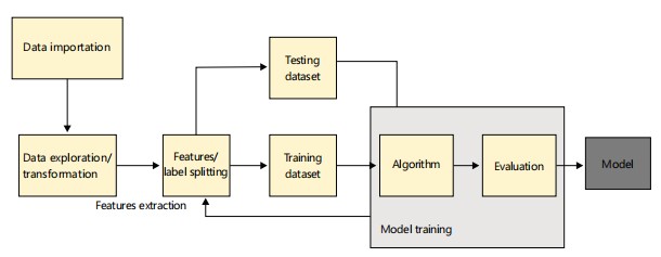
The workflow is detailed in Fig. 1, It follows the conventional workflow for machine learning prediction which involves importation of the dataset, extraction of meaningful information such as statistical information through transformation and/or exploration of the dataset, followed by partitioning of the data into features and labels. The data is further divided into training and testing set after which models are trained and evaluated. The process is repeated until a more suitable result is achieved.

Study duration: This research project was conducted from 6th August, 2024, to 12th February, 2025.

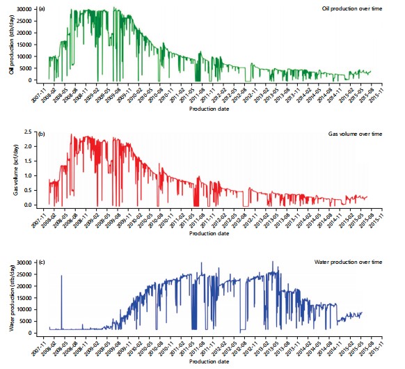
Dataset analysis: The dataset used in this research analysis contains five wells. The wells are combined to form custom data that was used in training the ML model. The custom dataset has 8 features and 3 production columns, which include oil, gas, and water production (Fig. 2a-c shows the production volume for 8 years) with a total of 6926 data observations.

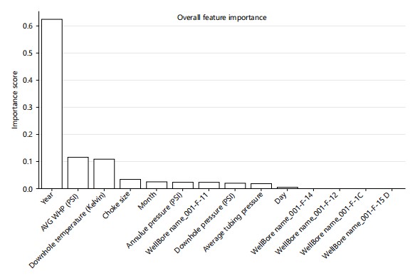
Feature column includes: Production Date (which was formatted into year, month, and day as separate columns), Well Bore Name, Downhole Pressure (PSI), Downhole Temperature (Kelvin), Average Tubing Pressure, Annulus Pressure (PSI), AVG WHP (PSI), and Choke Size. The production column (target) includes Oil Production (stb/day), Water Production (stb/day), and Gas Volume (scf/day). The significance of each of the features was evaluated using a random forest. The year was observed to be of utmost importance, as shown in Fig. 3. This affirms the time-dependent nature of the dataset utilized the following model in this prediction analysis.

Standalone model
Multiple linear regression: Multiple Linear Regression (MLR) is generally used to find the relationships of a dependent variable with numerous independent or predictive factors¹. It is an extension of simple linear regression, which only considers one independent variable. The model employs a linear regression framework, wherein the input features are linearly combined using coefficients estimated through optimization techniques, such as Ordinary Least Squares (OLS)¹³, to predict the continuous output variable to predict the continuous output variable. Multiple Linear Regression (MLR) establishes a mathematical relationship between multiple input variables (xn) and a target variable (y), as described by equation:

y = w0+w1×1+…+wnxn

(1)

Where:

	y	=	Dependent variable
	w0	=	Intercept
	w0 and wn	=	Coefficients for the independent variables
	x1 and xn	=	Independent variables

Fig. 1: Analysis workflow

Given data xi ∈ Rd, yi ∈R are the input features and the target values, respectively. The function is represented as:

f(x) = wT(x)+b

(2)

Where:

	wT	=	Weight vector
	x	=	Input feature vector
	b	=	Bias term

Radial basis function (RBF) was utilised in our research analysis. The equation is represented as:

K(xi,xj) = exp(-γ||xi-xj||2)

(3)

Where:

	xi and xj	=	Two feature vectors
	||xi-xj||2	=	Squared Euclidean distance between the vectors
	γ	=	Hyperparameter that defines how far the influence of a single training sample reaches

Support vector regression (SVR): The SVR is a sophisticated and popular ML algorithm that is generally considered an extension of support vector classification, which in turn is believed to be an extension of the perceptron. Support Vector Machines (SVM) involves the transformation of a low-dimensional, non-linear data to a higher-dimensional feature space, where the problem becomes linearly separable¹⁴.

Decision tree regression (DTR): The DTR is an ML algorithm that predicts continuous outcomes. It works by creating a tree-like network, where internal nodes denote features or attributes; branches denote decisions or splits; leaf nodes represent predicted outcomes¹⁵. A regression tree is generally more intricate than a classification tree. In decision tree regression, the data is optimally divided into segments known as leaves.

Fig. 2(a-c): Production volume through the years, (a) Oil production, (b) Gas volume and (c) Water production

This division is achieved by utilizing threshold values to address two key questions: i. Does splitting a node in a decision tree provide additional insights into the dataset? ii. Does incorporating information entropy provide any additional value to the method we intend to use for grouping our data points? [1] The algorithm stops when a stopping criterion is reached¹⁶.

The predicted outcome is the average value of the target variable in each leaf node.

The outcome is predicted as the average value of the target variable in each leaf node with equation:

(4)

Where:

	Ȳ	=	Predicted value for input x
	Yi	=	Actual target values
	n	=	Number of samples

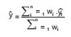
RFR: Random Forest Regression (RFR) is an ML-based regression technique that draws on the power of bagging and random subspace methods¹⁷. It generates a diverse ensemble of decision trees through bagging, which combines multiple trees to produce a single, robust prediction. To train the individual trees, the algorithm produces numerous bootstrap samples by resampling the original training data, each consisting of N instances randomly selected with replacement. The overall prediction is then obtained through a combination of these tree predictions, as represented by the general equation for RFR prediction:

(5)

Where, , K, h_k, denote the final predicted continuous value, the number of trees in the forest, and the numeric output from the i^th tree for input (x), respectively

XGBoost: The XGBoost is an optimized gradient-boosted decision tree (GBM) algorithm that balances performance and speed. It employs gradient tree boosting and offers various features to enhance its functionality. Unlike standard optimization methods, XGBoost uses an incremental approach to train the model, as traditional methods cannot improve the tree ensemble in Euclidean space¹⁷. Regularized learning is also utilized to smooth the final learned weights, preventing overfitting due to dataset size and other factors. The regularized objective favors models with simple and predictive functions¹⁷.

The XGBoost is particularly useful if the number of features is reduced compared to the number of observations or when dealing with numeric features exclusively. It operates similarly to a decision tree, creating a specific number of trees based on the problem, but does so incrementally. Each new tree compensates for the errors from the prior tree, allowing for improved performance. The XGBoost underhood is represented as:

(6)

Where:

	Yi	=	Predicted value for the ith value
	XI	=	Field vector of the ith data point
	fd	=	nth regression tree
	N	=	Total iteration
	F	=	Space of all possible regression trees

ANN: An Artificial Neural Network (ANN) is a deep learning method that mimics the human brain’s functionality by simulating the interactions between neurons¹⁸. It consists of three primary layers: an input layer, one or more hidden layers, and an output layer. The input layer receives and processes datanet inputs, assigning weights and passing them to the hidden layers, where complex representations are built through the application of activation functions and bias variables. Each hidden layer can employ different activation functions, allowing for diverse transformations of the data. Ultimately, the outputs from all hidden layers are aggregated in the output layer, where the final predictions are made, such as forecasting oil, gas, and water production over three years in our experiment, which utilized 35 output neurons. At its core, ANN relies on a network of interconnected neurons across multiple layers, receiving inputs (xi) with associated weights (wij) and bias values, enabling the activation function to be shifted by a constant¹⁹, as represented in Equation (8).

(7)

Where:

	Nj	=	Output of hidden neuron j
	σ	=	Output activation function
	wij	=	Weight from input neuron j
	xi	=	Input features
	bj	=	Bias for hidden neuron j

Rotation forest (PCA with random forest as the base model): It employs feature extraction and rotation to generate diverse base classifiers, resulting in a robust ensemble framework. The central idea of Rotational forest is to apply rotation to the feature space. This is achieved through Principal Component Analysis (PCA) or other linear transformations on random subsets of the features^20,21.

Each subset is transformed independently, ensuring that the rotated feature sets are unique for each base classifier.

Rotational forest constructs an ensemble of the base learners. The base learners are trained on a different rotated version of the data²¹. The rotations increase the diversity among base classifiers, which is critical for reducing the risk of overfitting and improving generalization²¹

Steps in rotational forest with random forest as base model
Dataset partitioning: The feature set X with n features is divided into K non-overlapping subsets. For instance:

if X = {x1, x2,… , xn}

(8)

It is partitioned into K subsets, such as S1, S2, . . ., SK, where

(9)

Feature rotation

	•	For each subset Sk
	•	Perform PCA to extract principal components
	•	Retain all principal components to ensure no information loss
	•	Use the rotation matrix obtained from PCA to transform the subset
	•	Rotated feature subsets are concatenated to form a transformed feature set for training the base model

Training base models: Train a separate base model on each transformed dataset created through PCA-based rotation. In the case of this analysis, a random forest was used as the base model.

Since Random Forest uses bagging and feature randomization, the rotational transformation further increases diversity among the decision trees.

Novel ensemble model
Stacked model: Stacked modeling, or stacking, utilizes a meta model to combine or stack various models’ predictions to improve overall performance. Introduced by Wolpert²², stacking operates on the principle that individual models may specialize in mapping different patterns present in the data, including the collective outputs can provide a more robust and precise prediction. The key idea is to use a model denoted as the meta-learner to learn the best techniques in combining the predictions of the prior models.

Stacking is highly versatile and can be applied to both classification and regression tasks. Unlike simple averaging or voting ensemble methods, stacking explicitly learns the optimal way to combine model outputs, which often results in superior predictive performance.

Weighted average ensemble: Weighted average ensembles operate on the assumption that certain models within the group possess greater accuracy or skill compared to others, and thus, these models are assigned a higher weight or contribution when making predictions. It is a robust ensemble modelling technique used in improving predictive performance by combining the outputs of multiple base models. Each model contributes to the last prediction based on a pre-assigned weight, reflecting its performance or reliability.

(10)

Where:

	y	=	Final ensemble prediction
	n	=	Number of models in the ensemble
	wi	=	i-th model, and denotes the prediction of the i-th model.
	wi	=	Weights wi are often normalized to sum up to 1, making the denominator

In this case, the formula simplifies to:

(11)

This analysis aims to predict three variables: Petroleum production; therefore, a Multiple Output regression was utilized for the model.

Model performance evaluation index: Three models are selected to evaluate the model’s performance. They include: i.) Root mean squared error (RMSE), ii.) Mean absolute error (MAE), iii.) Determination coefficient (R2). Equations for calculating the indices are as follows:

(12)

(13)

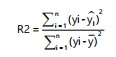(14)

Where:

	yi, l,	=	Actual values, prediction values and mean values of the sample data, respectively
	n	=	Sample size

Greater R2 score (tending to 1) and smaller RMSE and MAE score denotes better performance

Data preprocessing: An 80% training data with 20% testing data split achieved with the sklearn train_test_split library was utilized. Standardization was applied to the dataset. The sklearn StandardScaler was used to normalize the dataset. Additionally, a Multi-Output regression model was used to predict the three variables simultaneously. The parameters used in all the models we utilized for this prediction purpose are represented in Table 1.

RESULTS

Standalone model
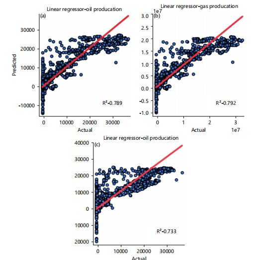
Multiple linear regression (MLR): Sklearn Linear Regression was used in implementing the multiple linear regression model. Figure 4a-c shows the distribution plot of the prediction against the real values. for oil production, gas production, and water production prediction, the R2 obtained are 0.789, 0.792, and 0.733 respectively.

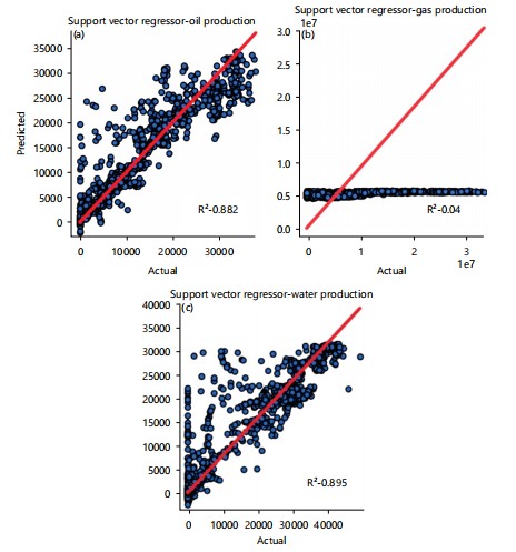
SVR: The dataset was normalized using the sklearn StandardScaler() library. Grid search was applied to obtain the best hyperparameter. The hyperparameter that yields the best outcomes can be seen in Table 1. The distribution plot of the actual and predictions of petroleum production is visualized in Fig. 5a-c. 0.882, 0.04, and 0.895 are the R2 scores obtained for oil production, gas production, and water production, respectively.

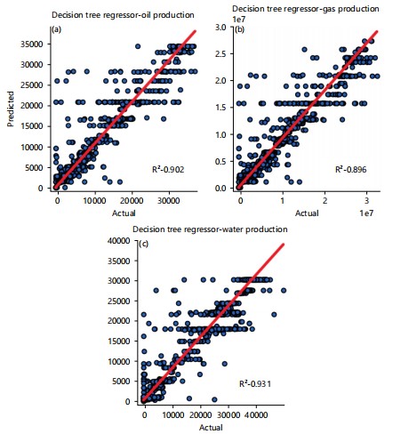
DTR: Decision Tree Regression (DTR) algorithm from sklearn. tree was applied in this model. The dataset was standardized and normalized. Grid search techniques were also applied for hyperparameter tuning. The following hyperparameters produced the best results: max_depth ‘7’, min_samples_leaf ‘10’. Figure 6a-c shows the plot of predictions versus the actual values for oil production, gas production, and water production achieved an R2 score of 0.902, 0.895, and 0.931, respectively.

Fig. 3: Features importance

Fig. 4(a-c): A distribution plot of MLR prediction values and the actual value of the three productions, (a) Oil production, (b) Gas production and (c) Water production

Table 1:

Parameters and hyperparameters used for different machine learning models employed in the prediction task after preprocessing with 80:20 train-test split and standardization

Model	Parameter	Parameters value
MLR	-	-
SVR	Kernel	rbf
	Gamma	auto
	C	2000
	Epsilon	0.01
DTR	Max_depth	7
	Min_samples_leaf	10
RFR	N_estimator	100
	Random_state	42
XGBoost	Objective	Reg:squarederror
	n_estimators	200
	Random_state	42
Rotational forest (pca + random forest)	No. of subset	3
	For the base model
	N_estimator	100
ANN	Optimizer	adam
	Dense	64
	Drop-out	0.2
	Activation	relu
	Epochs	200
	Batch-size	32
	Validation_split	0.2

Fig. 5(a-c): A distribution plot of SVR predictions values and actual value of the three productions, (a) Oil production, (b) Gas production and (c) Water production

Table 2:

Weight assigned to the models

Models	Oil production prediction	Gas production prediction	Water production prediction
Random forest	0.3348312	0.3357409	0.3335228
Xgboost	0.3326797	0.3326797	0.3336593
ANN	0.3326074	0.3315793	0.3328179

Table 3:

Determination coefficient (R2) score (the highest values were highlighted)

Model	Oil production	Gas production	Water production	Average score
MLR	0.789	0.792	0.733	0.771
SVR	0.871	-0.016	0.871	0.575
DTR	0.902	0.896	0.931	0.91
ROT RF	0.944	0.941	0.951	0.945
XGB	0.942	0.939	0.965	0.949
ANN	0.948	0.943	0.963	0.951
RF	0.949	0.948	0.964	0.954
Stacked	0.941	0.94	0.964	0.948
WE	0.952	0.951	0.97	0.958

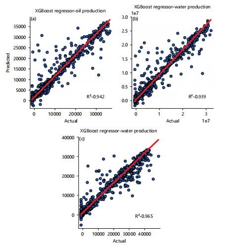
XGB: The XGBoost library was used in the implementation of this model-XGBoost (XGB). Standardization and normalization were implemented for this model. Grid search was also applied. The best result was achieved with the following hyperparameters: Objective ‘reg:squarederror’; colsample_bytree ‘0.3’; n_estimators ‘200’, random_state 42. Oil, water, and gas production prediction attained an R2 of 0.942, 0.939, and 0.964, respectively. Figure 7a-c is a plot showing the distribution of predicted values against the actual values.

Fig. 6(a-c): A distribution plot of DTR predictions and the actual value of the petroleum production, (a) Oil production, (b) Gas production and (c) Water production

Table 4:

MAE and RMSE score (The highest values were highlighted)

	MAE score			RMSE score
Model	Production oil	Production for gas	Production for water	Production oil	Production for gas	Production for water
MLR	2735.21	2123914.1	4379.46	4097.12	3232452.6	5972.47
SVR	1625.72	4993338.9	2167.48	3206.08	7145420.5	4151.7
DTR	1324.43	1090164.1	1544.46	2793.49	2289331.2	3026.37
XGB	777.91	654773.81	958.04	2144.14	1747492.5	2173.48
RFR	705.57	580100.69	816.34	2021.09	1618460.7	2185.58
ANN	1037.61	918518.38	1153.24	2031.49	1696972.3	2212.64
ROT RF	772.45	646464.87	998.14	2118.19	1718258.8	2552.22
Stacked	780.31	650043.37	973.07	3206.08	7145420.5	4151.7
WE	756.19	642692.66	871.73	1947.37	1568563.9	1987.4

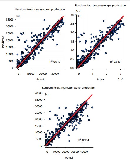
RFR: Random Forest Regression (RFR) model from sklearn. The ensemble was implemented. Standardization and normalization were applied to the dataset. A grid search technique was also implemented for hyperparameter tuning. The best result was obtained with the following hyperparameters: n_estimators ‘100, random_state = 42. The most outstanding evaluation score for the standalone model was achieved with this model. For oil, gas, and water production, a better R2 score of 0.948, 0.947, and 0.964 was achieved. Figure 8, shows the plot of production prediction versus real values. The points are tightly clustered around the red line, which shows a high level of prediction accuracy.

Fig. 7(a-c): A distribution plot on XGB predictions and actual value of the petroleum production, (a) Oil production, (b) Gas production and (c) Water production

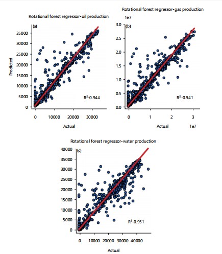
Rotational forest model: Feature transformation (feature extraction and rotation) was applied using PCA from sklearn. Decomposition and random forest regression as base learner. The parameters of the base learner include n_estimator: 200, random_state: 42. Three random subsets were used in this prediction. This model, for oil, gas, and water produced, had R2 score of 0.924, 0.926, and 0.950, respectively. Figure 9, Shows the distribution plot of the prediction values versus real values.

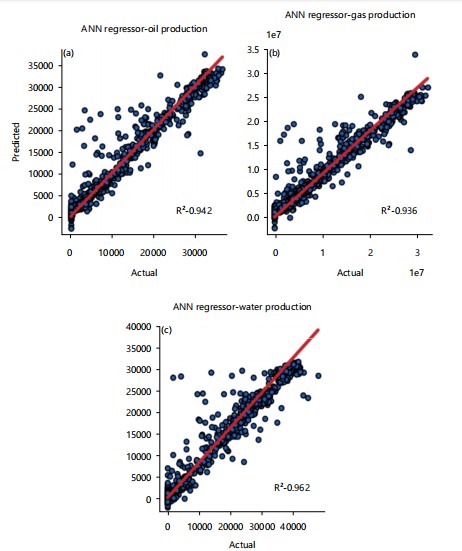
ANN: For Artificial Neural Network (ANN), a Sequential classifier from keras. The models library was used in building this model. Standardization and normalization were applied to the data set. The hyperparameters that were adopted in this prediction process are recorded in Table 1. The deep learning algorithm for oil, gas, and water production prediction attained an R2 score of 0.942, 0.936, and 0.962, respectively, as shown in Fig. 10.

Novel ensemble model
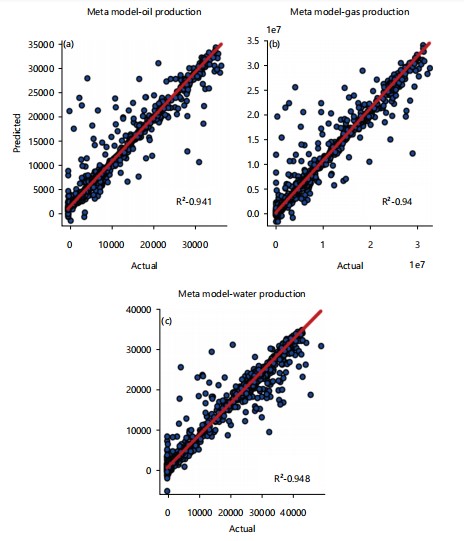
Stacked model: Predictions of random forest, Xgboost, and artificial neural network (which are the top-performing standalone models) were stacked together with the numpy column_stack function. A linear model was used as the meta model to map the linear relationship between the predictions. For oil, gas, and water production prediction, good R2 scores of 0.941, 0.939, and 0.963 were achieved. Fig. 11. shows the p lot of production prediction values versus the real values.

Fig. 8(a-c): A distribution plot of RFR prediction values and the actual values of the three production, (a) Oil production, (b) Gas production and (c) Water production

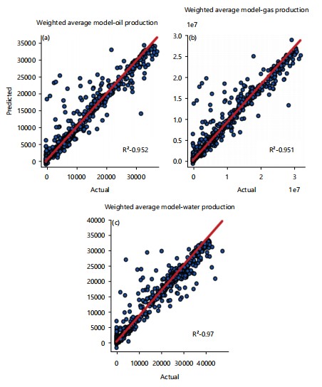
Weighted average: Weights were assigned to three models, which are random forest, xgboost, and artificial neural network. More weight was assigned to the random forest model with an average weight of 0.3347, which is the highest among the three models. 0.333 and 0.332 were assigned to XGBoost and ANN, respectively (shown in Table 2). The weighted average model has an outstanding average R2 score of 0.956. Oil production prediction has an R2 score of 0.951, 0.948 and 0.970 for gas and water production prediction, respectively (Fig. 12). In comparison to other ensemble and standalone models weighted average has an outstanding prediction performance.

The standalone model had the least performance on the gas production prediction, except for multiple linear regression, which had its least performance for oil production prediction, as seen

Fig. 9(a-c): A distribution plot on rotational forest predictions and actual value of the three production, (a) Oil production, (b) Gas production and (c) Water production

in Table 3. Random forest regression has the best performance among the standalone models, the highest R2 average score of 0.953, and the least MAE, RMSE, and MSE scores. For the novel ensemble model weighted average model has the best performance with an average R2 score o f 0.957 (Table 3), and the lowest error scores. Overall, the weighted average model outperformed other models. It achieved the highest R2 score (Table 3) and the lowest error score (Table 4) except for mean absolute e rror, w here random forest has the least error score. For R2 score, the weighted average model outperformed random forest by 0.42%, also ANN, XGBoost, stacked model, rotational forest, DTR, MLR and SVR were outperformed by 0.73, 0.93, 1.04, 1.35, 5, 19 and 39% respectively well, with support vector regression having the least performance (an average R2 score of 0.606 and highest error score) this is due to extremely poor prediction. the weighted approach optimizes overall accuracy by strategically blending predictions. This ensemble method typically achieves better generalization by balancing underfitting/overfitting risks across diverse data patterns.

Fig. 10(a-c): A distribution plot of ANN predictions and actual values of the three production, (a) Oil production, (b) Gas production and (c) Water production

DISCUSSION

This analysis highlights the efficacy of ensemble machine learning techniques in petroleum production prediction. The weighted average ensemble model outperformed standalone models in predicting petroleum production (oil, gas, and water). It achieved an average R² score of 0.958 and the lowest RMSE values. Random Forest Regression (RFR) has demonstrated the strongest performance among standalone models, with R² score of 0.953, which is followed by XGBoost (R² score of 0.949) and Artificial Neural Networks (R² score of 0.951). These findings showcase the superiority of the novel ensemble methods in capturing complex, nonlinear relationships inherent in petroleum production data. These align with the growing emphasis on data-driven decision-making in the oil and gas industry.

The results highlighted the robustness of ensemble methods in handling imbalanced geoscientific datasets. This is in agreement with Jamshidi Gohari et al.⁹. Their work emphasized that combining multiple base learners mitigates overfitting, a trend observed in our weighted average ensemble. The exceptional performance of RFR also aligns with Breiman¹⁷, who established its efficacy in noisy datasets. Similarly, Ibrahim et al.¹ reported RFR as the top performer in hydrocarbon production forecasting, attributing its success to feature randomization and bagging. Our stacked model (R²= 0.948) did not surpass RFR, contrary to Wolpert’s²² hypothesis that meta-learners enhance predictions. This suggests that simpler ensemble methods (e.g., weighted averaging) may be more effective for petroleum production datasets. Further experimenting may provide more balance and distinctions between the two methods.

Fig. 11(a-c): A distribution plot of the stacked model’s actual predictions and actual values of the three production, (a) Oil production, (b) Gas production and (c) Water production

The dataset is a major limitation to this analysis. It comprised only five wells. This may limit the individual model's generalization ability. Future work should incorporate larger, geographically diverse datasets. The models were tested on historical data, integration of real-time sensor data, as proposed by Nautiyal and Mishra¹², could improve dynamic forecasting. Ensemble models sometimes lack interpretability. Hybrid approaches, which combine ML with physics-based model² could bridge this gap.

Fig. 12(a-c): A distribution plot on weighted average model’s predictions and actual values of the three productions, (a) Oil production, (b) Gas production and (c) Water production

CONCLUSION

This study applied standalone and ensemble machine learning models to predict oil, gas, and water production. Among the standalone models, rotational forest, XGBoost, ANN, and random forest demonstrated strong performance with average R² scores of 0.932, 0.948, and 0.953. The weighted average ensemble achieved the best results overall, with the highest R² score of 0.956 and the lowest RMSE. Although the stacked model combining random forest, XGBoost, and ANN did not surpass the best standalone models, further optimization could enhance its effectiveness. Overall, the findings highlight the value of artificial intelligence in petroleum production forecasting, offering a sustainable, accurate, and cost-effective approach for the oil and gas industry.

SIGNIFICANCE STATEMENT

Accurate forecasting of petroleum prediction is critical for optimizing resource management and planning in the oil and gas industry, yet traditional prediction methods often fall short in capturing the complex relationships among production parameters. This study developed and compared seven advanced machine learning models and introduced ensemble approaches-specifically a weighted average ensemble of Random forest, XGBoost, and Artificial Neural Network-to predict oil, gas, and water production rates.

The weighted ensemble model significantly outperformed all others, achieving an R² score of 0.949 for oil, 0.948 for gas, and 0.968 for water, averaging 0.958, alongside the lowest RMSE values. These results underscore the superior accuracy and robustness of ensemble machine learning methods, particularly weighted averaging, over individual and stacked models. This advancement offers substantial potential to enhance data-driven decision-making and operational efficiency across petroleum exploration and production activities globally.

REFERENCES

1. Ibrahim, N.M., A.A. Alharbi, T.A. Alzahrani, A.M. Abdulkarim and I.A. Alessa et al., 2022. Well performance classification and prediction: Deep learning and machine learning long term regression experiments on oil, gas, and water production. Sensors, 22.
2. Islam, M.R., M.E. Hossain, S.H. Moussavizadegan, S. Mustafiz and J.H. Abou-Kassem, 2016. Reservoir Simulator-Input/Output. In: Advanced Petroleum Reservoir Simulation: Towards Developing Reservoir Emulators, Islam, M.R., M.E. Hossain, S.H. Moussavizadegan, S. Mustafiz and J.H. Abou-Kassem (Eds.), Wiley, New Jersey, ISBN: 9781119038573, pp: 39-84.
3. Hastie, T., R. Tibshirani and J. Friedman, 2009. The Elements of Statistical Learning: Data Mining, Inference, and Prediction. 2nd Edn., Springer, New York, ISBN: 978-0-387-84858-7, Pages: 745.
4. Bishop, C.M., 2006. Pattern Recognition and Machine Learning. 1st Edn., Springer, Heidelberg, ISBN: 978-1-4939-3843-8, Pages: 778.
5. Tang, Y., J. Kurths, W. Lin, E. Ott and L. Kocarev, 2020. Introduction to focus issue: When machine learning meets complex systems: Networks, chaos, and nonlinear dynamics. Chaos: Interdiscip. J. Nonlinear Sci. 30.
6. Cenedese, M., J. Axås, B. Bäuerlein, K. Avila and G. Haller, 2022. Data-driven modeling and prediction of non-linearizable dynamics via spectral submanifolds. Nat. Commun., 13.
7. Elmabrouk, S., E. Shirif and R. Mayorga, 2014. Artificial neural network modeling for the prediction of oil production. Pet. Sci. Technol., 32: 1123-1130.
8. Negash, B.M. and A.D. Yaw, 2020. Artificial neural network based production forecasting for a hydrocarbon reservoir under water injection. Pet. Explor. Dev., 47: 383-392.
9. Gohari, M.S.J., M.E. Niri, S. Sadeghnejad and J. Ghiasi-Freez, 2023. An ensemble-based machine learning solution for imbalanced multiclass dataset during lithology log generation. Sci. Rep., 13. https://doi.org/10.1038/s41598-023-49080-7
10. Roncoroni, G., E. Forte and M. Pipan, 2024. Deep attributes: Innovative LSTM-based seismic attributes. Geophys. J. Int., 237: 378-388.
11. Yu, S. and J. Ma, 2021. Deep learning for geophysics: Current and future trends. Rev. Geophys., 59.
12. Nautiyal, A. and A.K. Mishra, 2022. Machine learning approach for intelligent prediction of petroleum upstream stuck pipe challenge in oil and gas industry. Environ. Dev. Sustainability.
13. Chen, Y., X. Ding, H. Liu and Y. Yan, 2013. Comparisons of oil production predicting models. Engineering, 5: 637-641.
14. Seal, H.L., 1967. Studies in the history of probability and statistics. XV the historical development of the Gauss linear model. Biometrika, 54: 1-24.
15. Wei, W., X. Li, J. Liu, Y. Zhou, L. Li and J. Zhou, 2021. Performance evaluation of hybrid WOA-SVR and HHO-SVR models with various kernels to predict factor of safety for circular failure slope. Appl. Sci., 11.
16. Shalev-Shwartz, S. and S. Ben-David, 2014. Decision Trees. In: Understanding Machine Learning: From Theory to Algorithms, Shalev-Shwartz, S. and S. Ben-David (Eds.), Cambridge University Press, Cambridge, United Kingdom, ISBN: 9781107298019, pp: 212-218.
17. Breiman, L., 2001. Random forests. Mach. Learn., 45: 5-32.
18. Pesantez-Narvaez, J., M. Guillen and M. Alcañiz, 2019. Predicting motor insurance claims using telematics data-XGBoost versus logistic regression. Risks, 7.
19. Goodfellow, I., Y. Bengio and A. Courville, 2016. Deep Learning. MIT Press, Cambridge, Massachusett, ISBN: 9780262035613, Pages: 775.
20. LeCun, Y., Y. Bengio and G. Hinton, 2015. Deep learning. Nature, 521: 436-444.
21. Rodriguez, J.J., L.I. Kuncheva and C.J. Alonso, 2006. Rotation forest: A new classifier ensemble method. IEEE Trans. Pattern Anal. Mach. Intell., 28: 1619-1630.
22. Wolpert, D.H., 1992. Stacked generalization. Neural Networks, 5: 241-259.