Modeling and Short Term Forecasting of Wind Speed Potentials for the Generation of Electricity for Nigerian Army University Biu

Received 29 Aug, 2019

Accepted 15 Dec, 2019

Published 15 Jan, 2020

ABSTRACT

Background and Objectives: Wind energy is the natural air that flows through the wind turbine which provides mechanical power and turns to electrical generator. Current research proposed a model and forecast wind speed potentials for the generation of electricity for Nigerian Army University Biu and following challenges were addressed, wind speed potentials of Biu town was modeled, characterized, forecasted and also the effects of temperature and relative humidity on the wind speed were examined. Materials and Methods: Weibull model was employed to model and characterize the hourly average wind speed measured at 10 and 80 m for one week from 9^th-15^th June, 2019. Neuro-fuzzy hybrid model was used to forecast the hourly average wind speed. Results: The results show that the hourly average wind speed measured at 10 m was 2.58 ms^-1 and at 80 m was 3.56 ms^-1 and, the forecasted was 2.68 ms^-1 and 3.61 ms^-1, respectively. It was expected that the wind speed will increase by 5-12% on the 9^th-15^th June, 2020 and is adequate to turn the wind turbine especially at 80 m. It was examined that as temperature increases wind speed reduces, whereas the relative humidity does not show notable effect. Conclusion: Wind power can be an alternative source of power for the generation of electricity for Nigerian Army University Biu. It is further recommended that long term forecasting may be applied to assess the wind speed potentials for the remaining months and turbine higher 80 m may be required to enhance better performance.

INTRODUCTION

It is expected that the cost of installing, operating and maintenance of Wind Power Plant (WPP) is far less than that of Hydro Power Plant (HPP) mostly used as a source power in Nigeria. The HPP are usually installed where there is Rivers/water fall before the power can be generated and transmitted to the consumer's over a considerable distance¹. These processes may not be hitched free from regular power outages and huge energy losses². Its capacity highly depends on the volume of water discharge by the river unlike wind energy that is abundant and readily available all over the country. The demand of alternative sources of energy for generation of electricity has become paramount in order to supplement the limited energy generated by the different power companies in Nigeria³. Many power consumers believed to date that in future the Megawatt presently in use may not sufficiently meet their needs due to the rapid growing of Nigerian population and the continued industrialization⁴. For example, China, Germany, USA, Brazil, India, Canada, United Kingdom, Sweden and France have generated up to 22,482 MW, 4,410 MW, 3,9854 MW, 1,603 MW, 14,46 MW, 1,002 MW, 867 MW, 181 MW and 173 MW, respectively. In fact, the country needs to adopt wind power as an alternative source of energy for the generation of electricity. In addition, United Nations Frame Work Convention on Climatic Change (UNFCCC), Clean Development Mechanism Executive Board (CDM–EB) and United Nation Environmental Program (UNEP) have reported several times that there is a need to change to energy production and utilization practices because of the raising alarm in climatic change pattern across the globe which may result to persistent drought⁵. This entails that HPP may not be reliable source of power in Nigeria in future.

Works have been intensively conducted on this field by different authors for instance^6–15. Sarkar et al.¹⁶ analyzed wind power potentials in three locations in the South East of Nigeria and, determined that the average monthly wind speed ranges from 3.36-5.42 ms^-1 Merovci and Elbatal¹⁷ statistically analyzed wind speed using Weibull, Rayleigh and Gamma distributions for the generation of electricity in some selected sites in the Northern part of Nigeria and found that Weibull distribution is the best model. Topaloglu and Pehlivan¹⁸ investigated wind speed potentials using Weibull, Rayleigh and cumulative distribution functions and arrived at wind speed from January-December ranges from 3.88-8.47 ms^-1 and, adequate for generation of electricity. Danladi et al.¹⁹, applied Weibull model to determine wind speed pattern in some coastal and inland areas of Nigeria and obtained that wind speed is adequate for the generation of electricity in these areas. All authors did not forecast to know the wind speed condition in future.

Current research proposed model, which forecast and examine the effects of climatic change on the wind potentials for the generation of electricity for Nigerian Army University Biu while following were the objectives of this study: to model and characterize the wind speed potentials of Biu town, forecast the wind speed of 9^th-15^th June, 2020 and examine the effects of temperature and relative humidity.

MATERIALS AND METHODS

Study area and method of data collection: Biu lies on the Biu Plateau at an average elevation of 626 m, Latitude 10/61°N, Longitude 12.195°E and time zone UTC+1 (CET). The region is semi-arid. The satellite data of weather parameters was collected from the Meteoblue in Switzerland. The data include temperature, relative humidity and wind speed (WS) measured at 10 and 80 m, while the hourly average wind speed measured at 10 and 80 m for one week from 9^th-15^th June, 2019. The data shall be modeled and forecasted using Weibull and Neuro–fuzzy hybrid models, respectively.

Modeling of wind speed using Weibull model: Weibull Model (WM) is a probability distribution function model generally accepted for modeling of weather parameters especially solar radiation and wind power. The model equation is expressed as;

$$ \mathrm{f}(\mathrm{v})=\left(\frac{\mathrm{K}}{\mathrm{C}}\right)\left(\frac{\mathrm{V}}{\mathrm{C}}\right)^{\mathrm{K}-1} \exp \left[-\left(\frac{\mathrm{V}}{\mathrm{C}}\right)^{-\mathrm{K}}\right] \mathrm{k}>0, v>0 $$

where, k is the dimensionless shape parameter, c is the scale parameter and its cumulative distribution function is also given by;

$$ f(v)=1-\exp \left[\left(\frac{v}{c}\right)^{-K}\right] $$

The 'WM' is said to be desirable or fit to characterize 'WS' if it is positively sketched (i.e., when, k≤3.6). It becomes undesirable¹⁹, if k>3.6. Furthermore, special cases may be applied where k = 1 and k = 2, 'WM' is considered as Exponential and Rayleigh distributions respectively²⁰. In real life situation, k = 2 happens more frequently than k = 1 and its probability distribution function is expressed as²¹.

$$ f(V)=\left(\frac{2 V}{C^{2}}\right) \exp \left[-\left(\frac{V}{C}\right)^{-K}\right] $$

Differentiating Eq. 1 yields;

$$ \bar{v}=\int_{0}^{\alpha}\left[\left(\frac{K}{C}\right)\left(\frac{V}{C}\right)^{K-1} \exp \left[-\left(\frac{V}{C}\right)^{-K}\right]\right] \mathrm{d} v $$

Assume that, then expression in Eq. 4 reduces to Eq. 5 as;

$$ \bar{v}=\int_{0}^{\propto} x^{\frac{1}{k}} \exp ^{-x} d x $$

and expression in Eq. 5 can be further written in form of gamma function as;

$$ \Gamma(y)=\int_{0}^{\infty} e^{-x} x^{y-1} d x $$

If Eq. 5 and 6 have the same integrand and , then the 'WS' is characterized using Eq. 7;

$$ \mathrm{V}=\mathrm{c} \Gamma\left(1+\frac{1}{\mathrm{k}}\right) $$

It is important to note that 'WS' varies with height. Usually, 'WS' measure at 20-150 m above ground reference is good for decision making especially for installation of turbines and locations²².

Forecasting of wind speed using neuro'fuzzy hybrid model: Neuro-Fuzzy is a Hybrid Model (NFHM) that combines two artificial intelligent techniques (i.e., Fuzzy Logic Model (FLM) and Artificial Neural Network (ANN) as depicted in Fig. 1.

Fig. 1: Neuro-fuzzy hybrid model

where: I_i: Input vector matrices, FI: Fuzzified input, FIE: Fuzzy interference engine, FO: Deffuzified output, HL: Hidden layer, NO: ANN output, MSE: Mean square error, BP: Back propagation.

Fuzzification: Normally, the input vector matrices (I_i) are given arbitrary class labels such as; Low (L), Medium (M), High (H) with overlapping scales as Low to Medium (LM) Medium to and High (MH) etc. The 'I_i' are normalized in linguistic understanding as; measured Wind Speed (v), Temperature (t), Relative Humidity (r) which are further fuzzified as:

Lv = 3–9 kph, Mv = 8–16 kph and Hv = 15–26 kph Lt = 18- 6°C and Mt= 25–35°C Lr = 20–36%, Mr = 35–60% and Hr = 58–80%

(8)

Before they are mapped into a membership function (μ)²³.

Membership function: Membership function is a graphical way of representing the universe of discourse and it is classified in many ways which include asymmetric triangular, trapezoidal, gaussian and generic (μs), to mention but a few. In this work, generic (μ) was applied to map the input as given in Eq. 9;

$$ \operatorname{bell}(1, a, b, c)=\frac{1}{1+\left|\frac{I-c}{a}\right|^{2 b}} $$

where 'a' determines the width of the bell shape, 'b' is the positive integer, 'c' sets the center of the curve and 'I' is the universe of discourse²⁴.

Fuzzy rule base: Rule Base (RB) is usually formulated in expert domain using if-then statement and, about 2ⁿ = 2⁴ = 32 rules are formed in this work, see few examples below.

if t is H and r is L then v is L if t is L and r is H then v is H if t is M and r is M then v is M

Fuzzy inference engine (FIE): This layer accepts 'FI' and 'RB'. The 'RB' acts ''FI' using firing strength 'FS' before deffuzzification is performed. The 'FS' operates either on AND, OR or NOT with maximum of two inputs at a time to compute their 'μ' values and the result most lie²² between 0 and 1. This implies that each value of 'μ' must have absolute belongingness '1' or non-absolute belongingness '0'. In this work, the rules were fired using Eq. 10 and 11 depending on the condition applied at a time.

$$ \mathrm{FS}=\min \left(\mathrm{m}_{\mathrm{v} 1}(\mathrm{~A} 1)\right),\left(\mathrm{m}_{\mathrm{v} 2}(\mathrm{~A} 2)\right), \ldots \ldots,\left(\mathrm{m}_{\mathrm{Vn}}(\mathrm{An})\right) $$
$$ \mathrm{FS}=\max \left(\mathrm{m}_{\mathrm{V} 1}(\mathrm{~A} 1)\right),\left(\mathrm{m}_{\mathrm{v} 2,}(\mathrm{~A} 2)\right), \ldots . .\left(\mathrm{m}_{\mathrm{Vn}}(\mathrm{An})\right) $$

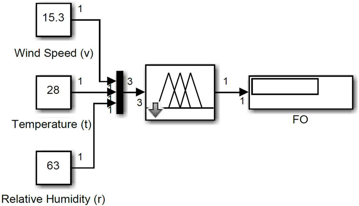
Deffuzzification: This is done by multiplying the combined control action of the 'FLM' as given in (Eq. 12)

$$ \mathrm{FO}=\frac{\sum_{\mathrm{i}=1}^{\mathrm{n}} \mathrm{FA}_{\mathrm{j}} \times \mathrm{Z}}{\sum_{\mathrm{i}=1}^{\mathrm{n}} \mathrm{FA}_{\mathrm{j}}} $$

where, 'FO' denotes the deffuzzified output (wind speed) as depicted in Fig. 2, FA_j is the firing areas of the j^th rule and Z is the centroid²⁵.

Fig 2: Fuzzy logic simulation model

Fig 3: Neutral network simulation model (H. Training and Back Propagation Algorithms)

The 'ANNM' receives the 'FO' as an input as shown in Fig. 3. This stage has no connecting nodes/weights nor activation function. It's only amplified the 'FO'. Furthermore, the 'ANNM' is trained and, the Hidden Layer (Hl) receives the amplified 'FO' (i=1,2,3,………n^th), connect it to the neurons Nj (j=1,2,3………..,n^th ) and then compute the 'NO' using Eq. 13-15.

$$ h_{\mathrm{j}}=\mathrm{f}\left(\sum_{n=1} \mathrm{~W}_{\mathrm{ij}} \mathrm{NO}_{\mathrm{i}}\right)+\mathrm{bW}_{\mathrm{oi}} $$

Where is f expressed as;

$$ f=\frac{1}{e^{-b j}} $$

f is the sigmoid function of the hidden layers (h_j) Whereas, the output of the hidden layer (NO)i is obtained by multiplying their connecting weight (Wi) plus bias (b) and the new weight is computed as;

$$ (\mathrm{NO})_{0-\mathrm{i}}=\sum_{\mathrm{i}=0}\left(\mathrm{~h}_{\mathrm{i}} \mathrm{w}_{\mathrm{i}}\right)+\mathrm{b} $$

where the output of the NFHM is determined using Eq. 16 given by;

$$ v_{f}=f_{0}(N O)_{0-i} $$

f_o is the linear transfer function and NO_0-1 is then compared with the target to give the forecasted wind speed (v_f). The error connecting the learning rule base after training²⁵ is obtained using Eq. 17.

$$ \operatorname{MSE}=\frac{1}{2}\left(\operatorname{target}-v_{f}\right) $$

RESULTS

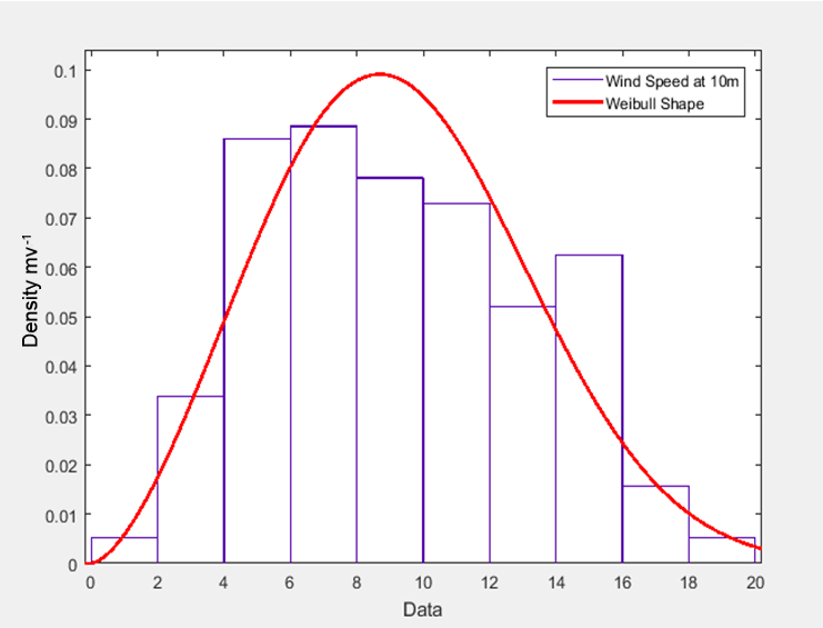
The results of the study have been presented in Fig. 4. Where, Fig. 4a shows the analysis of the 'WS' measured at 10 m using 'WM', Fig. 4b depicts the analysis of the 'WS' measured at 80 m using 'WM', Fig. 4c indicates the analysis of the 'WS' forecasted at 10 m using 'WM', Fig. 4d shows the analysis of the 'WS' forecasted at 80 m using 'WM' and Fig. 5 depicts the relationships between the temperature, relative humility, forecasted and measured 'WS' while the results of the analysis are summarized in Table 1-3.

Fig 4a. Analysis of 'WS' measured at 10 m

Fig 4b. Analysis of 'WS' measured at 80 m

Fig 4c. Analysis of 'WS' measured at 10 m

Fig 4d. Analysis of 'WS' measured at 80 m

Fig 5: Comparison of temperature, relative humility, forecasted and measured 'WS'

Table 1: Analysis of wind speed measured and forcasted using Weibull model
	WS (kph) at 10 m	WS (kph) at 80 m	WS (ms-1) at 10 m	WS (ms-1) at 80 m
c	10.50	4.42	2.90	4.01
k	2.59	2.42	-	-
v	-	-	2.56	3.56
cf	10.75	14.48	2,99	4.04
kf	3.16	2.92	-	-
vf	-	-	2.68	3.61
WS: Wind speed, C: Scale parameter, V: Wind speed Cf: Forcasted scale parameter, Kf: Forcasted shape parameter, Vf: Forcasted wind speed,

Table 2: Correlation coefficients between WS and weather parameters
Weather parameters	WS (ms-1) at 10 m	WS (ms-1) at 80 m
Temperature (°C )	- 0.38	- 0.62
Relative humidity (mm)	0.42	0.55

Table 3: MSE and NFM performances
	WS (ms-1) at 10 m	WS (ms-1) at 80 m	MSE	γ (%)
WS (ms-1) at 10 m	0.39	-	0.04	99.61
WS (ms-1) at 80 m	-	0.74	0.06	99.26
NFM: National utility financial model, MSE: Mean square error

Table 1 was derived from Fig. 4a-b, it shows the scale parameter (c), shape parameters (k) and wind shape 'v' is the average 'WS' measured at different heights. At 10 m: c = 10.50 kph (2.92 ms^-1), k = 2.59 and v = 2.58 ms^-1, at 80 m: c = 14.42 kph (4.01 ms^-1), k = 2.42 and v = 3.56 ms^-1 respectivel. The forecasted scale parameter (c_f), shape parameter (k_f) and wind speed (v_f) at different heights. At 10 m: c_f = 10.75 kph (2.99 ms^-1), k_f = 3.16 and v_f = 2.68 ms^-1. At 80 m: c_f = 14.41 kph (4.04 ms^-1), k_f = 2.92 and v_f = 3.61 ms^-1.

Table 2 was derived from the relationship between 'v' and 'v_f' with temperature and the relative humidity as depicted in Fig. 5. It can be seen that temperature (t) correlates negatively with 'v and v_f' at 10 and 80 m as -0.38 and -0.62 and relative humidity (r) correlates positively with 'v and v_f' at 0.42 and 0.55 respectively. In a nutshell, 'v and v_f' vary directly proportional to relative humidity and inversely proportional to temperature. Table 3 showed the MSE obtained between 'v' and 'v_f' at 10 and 80 m as 0.39 and 0.74, respectively. This confirms that the average performance of the NFHM is 99.44%.

DISCUSSION

The result presented in Table 1 is derived from Fig. 4a-b and it is in disagreement of what was presented by Ambach and Croonenbroeck¹⁴. 'k' is normally skewed in both scenarios and falls within the accepted modeling range 2.1≥k≤3.6. From these results, it is found that 'WM' is a good estimator of 'WS' and the average values of the 'WS' estimated at 10 and 80 m are adequate to turn Wind Turbine (WT) for the generation of electricity especially the 'WS'²⁴ measured at 80m. Additionally, the 'WS' at 80 m is greater than the minimum 'WS' required to turn the 'WT' by 1.14% and, its fall within the 'WT' survival velocity²⁴.

While result presented in Table 1 was obtained from Fig. 4c-d, shows the forecasted results, the average 'WS' at 10 and 80 m are also adequate to turn 'WT' for the generation of electricity for (NAUB) as reported also by Danladi et al.¹⁹ and in contrast to results obtained by Topaloglu and Pehlivan¹⁸. However, at 10 m: v_f> v by 0.12 ms^-1 and at 80 m: v_f> v by 0.05 ms^-1. This implies that in June, 2020 'WS' will increase by 12% and 5% at 10 and 80 m respectively. In general, it is observed that, both 'v' and 'v_f' increased with the increased in altitude²⁵.

In Table 2 results was derived from the 'v' and 'v_f' with temperature and the relative humidity which was presented in Fig. 5. This means that high temperature reduces 'WS' whereas relative humidity does not show any impact on the 'WS'²⁵.

CONCLUSION

Modeling and short term forecasting of the wind speed potentials for the generation of electricity for Nigerian Army University Biu was proposed in this work. Weibull model was employed to determine the average 'WS' measured at 10 and 80 m as 2.58 and 3.56 ms^-1, forecasted 'WS' as 2.68 and 3.61 ms^-1 respectively. It was found that 'WS' will increase from 5-12% from 9^th–15^th June, 2020 and 'WS' at 80 m is adequate to constantly turn the 'WT' since it falls slightly above the cut in speed. Relative humidity is directly proportional and temperature is inversely propositional to the 'WS'. Biu is a potential area for the generation of electricity using wind power. It is further recommended that long term forecasting shall be applied to forecast the 'WS' of the remaining months and turbine height of 80m may applied for better performance.

SIGNIFICANCE STATEMENT

This study uncovers that Hybrid fuzzy–neuro model significantly reduces 'WS' prediction errors than what is obtained using correlation, regression and other methods in literature. The study also revealed that 'WS' in Biu wind increase by 5-12% from 9^th-15^th June, 2020 and is adequate to turn the WT for the generation of electricity which can serve as an alternative source of power supply to the university. Also, the result of this study can serve a guide to the university whenever they wish to embark on wind speed power projects.

REFERENCES

1. Bhatti, S.S., M.U.U. Lodhi and Shan ul Haq, 2015. Electric power transmission and distribution losses overview and minimization in Pakistan. Int. J. Scient. Eng. Res., 6: 1108-1112.
2. Shalangwa, D.A., D.Y. Shinggu and T. Jonathan, 2009. An analysis of electric power faults in Mubi undertaking station, Adamawa State, Nigeria. Pac. J. Sci. Technol., 10: 508-513.
3. Shaaban, M. and J.O. Petinrin, 2014. Renewable energy potentials in Nigeria: Meeting rural energy needs. Renew. Sustain. Energy Rev., 29: 72-84.
4. Mazur, A., 1994. How does population growth contribute to rising energy consumption in America? Popul. Environ., 15: 371-378.
5. Petersen, E.L., 2017. In search of the wind energy potential. J. Renew. Sustain. Energy.
6. Celik, A.N., 2004. A statistical analysis of wind power density based on the Weibull and Rayleigh models at the Southern region of Turkey. Renew. Energy, 29: 593-604.
7. Azad, A.K., M.G. Rasul, M.M. Alam, S.M. Ameer Uddin and S.K. Mondal, 2014. Analysis of wind energy conversion system using Weibull distribution. Procedia Eng., 90: 725-732.
8. Saxena, B.K. and K.V.S. Rao, 2016. Estimation of wind power density at a wind farm site located in Western Rajasthan region of India. Procedia Technol., 24: 492-498.
9. Keyhani, A., M. Ghasemi-Varnamkhasti, M. Khanali and R. Abbaszadeh, 2010. An assessment of wind energy potential as a power generation source in the capital of Iran, Tehran. Energy, 35: 188-201.
10. Quan, P. and T. Leephakpreeda, 2015. Assessment of wind energy potential for selecting wind turbines: An application to Thailand. Sustain. Energy Technol. Assess., 11: 17-26.
11. Mirhosseini, M., F. Sharifi and A. Sedaghat, 2011. Assessing the wind energy potential locations in province of Semnan in Iran. Renew. Sustain. Energy Rev., 15: 449-459.
12. Santamaria-Bonfil, G., A. Reyes-Ballesteros and C. Gershenson, 2016. Wind speed forecasting for wind farms: A method based on support vector regression. Renew. Energy, 85: 790-809.
13. Mohandes, M., S. Rehman, M. Abido and S. Badran, 2016. Convertible wind energy based on predicted wind speed at hub-height. Energy Sources Part A: Recov. Utiliz. Environ. Eff., 38: 140-148.
14. Ambach, D. and C. Croonenbroeck, 2016. Space-time short-to medium-term wind speed forecasting. Stat. Methods Applic., 25: 5-20.
15. Doucoure, B., K. Agbossou and A. Cardenas, 2016. Time series prediction using artificial wavelet neural network and multi-resolution analysis: Application to wind speed data. Renew. Energy, 92: 202-211.
16. Sarkar, A., G. Gugliani and S. Deep, 2017. Weibull model for wind speed data analysis of different locations in India. KSCE J. Civil Eng., 21: 2764-2776.
17. Merovci, F. and I. Elbatal, 2015. Weibull Rayleigh distribution: Theory and applications. Applied Math. Inform. Sci., 9: 2127-2137.
18. Topaloglu, F. and H. Pehlivan, 2018. Analysis of wind data, calculation of energy yield potential and micrositing application with WAsP. Adv. Meteorol.
19. Danladi, A.D., M.I. Puwu, Y. Michael and B.M. Garkida, 2016. Use of fuzzy logic to investigate weather parameter impact on electrical load based on short term forecasting. Niger. J. Technol., 35: 562-567.
20. Danladi, A., M. Stephen, B.M. Aliyu, G.K. Gaya, N.W. Silikwa and Y. Machael, 2018. Assessing the influence of weather parameters on rainfall to forecast river discharge based on short-term. Alexandria Eng. J., 57: 1157-1162.
21. Danladi, A. and P.G. Vasira, 2018. Path loss modeling for next generation wireless network using fuzzy logic-spline interpolation technique. J. Eng. Res. Rep., 1: 1-10.
22. Ali, D., M. Yohanna, P.M. Ijasini and M.B. Garkida, 2018. Application of fuzzy-neuro to model weather parameter variability impacts on electrical load based on long-term forecasting. Alexandria Eng. J., 57: 223-233.
23. Anonymous, 2009. Wind turbine systems and renewable energy level.
24. Borsche, M., A.K. Kaiser-Weiss and F. Kaspar, 2016. Wind speed variability between 10 and 116 m height from the regional reanalysis COSMO-REA6 compared to wind mast measurements over Northern Germany and the Netherlands. Adv. Sci. Res., 13: 151-161.
25. Brower, M.C., M.S. Barton, L. Lledo and J. Dubois, 2013. Study of wind speed variability using global reanalysis data. AWS Truepower^®, Albany, NY., USA., May 2013, pp: 1-11.

This work is licensed under a Creative Commons Attribution 4.0 International License.